4 Getting acquainted
Let’s open RStudio and have a look around.
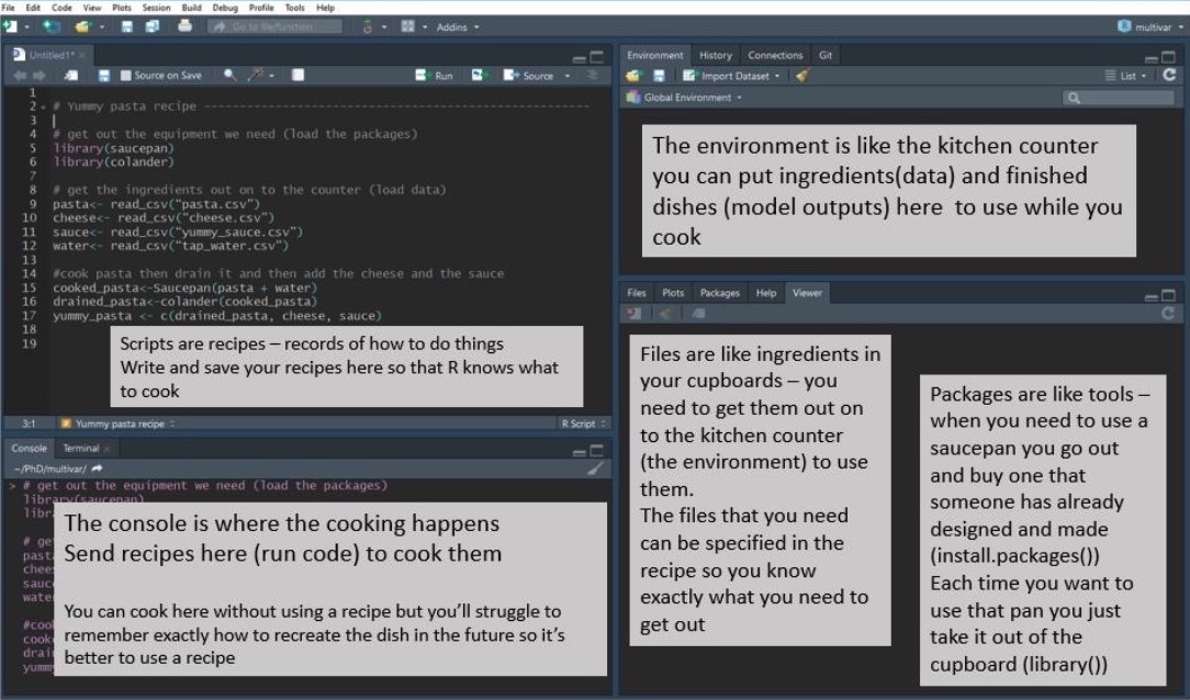
4.1 Finding your way around RStudio
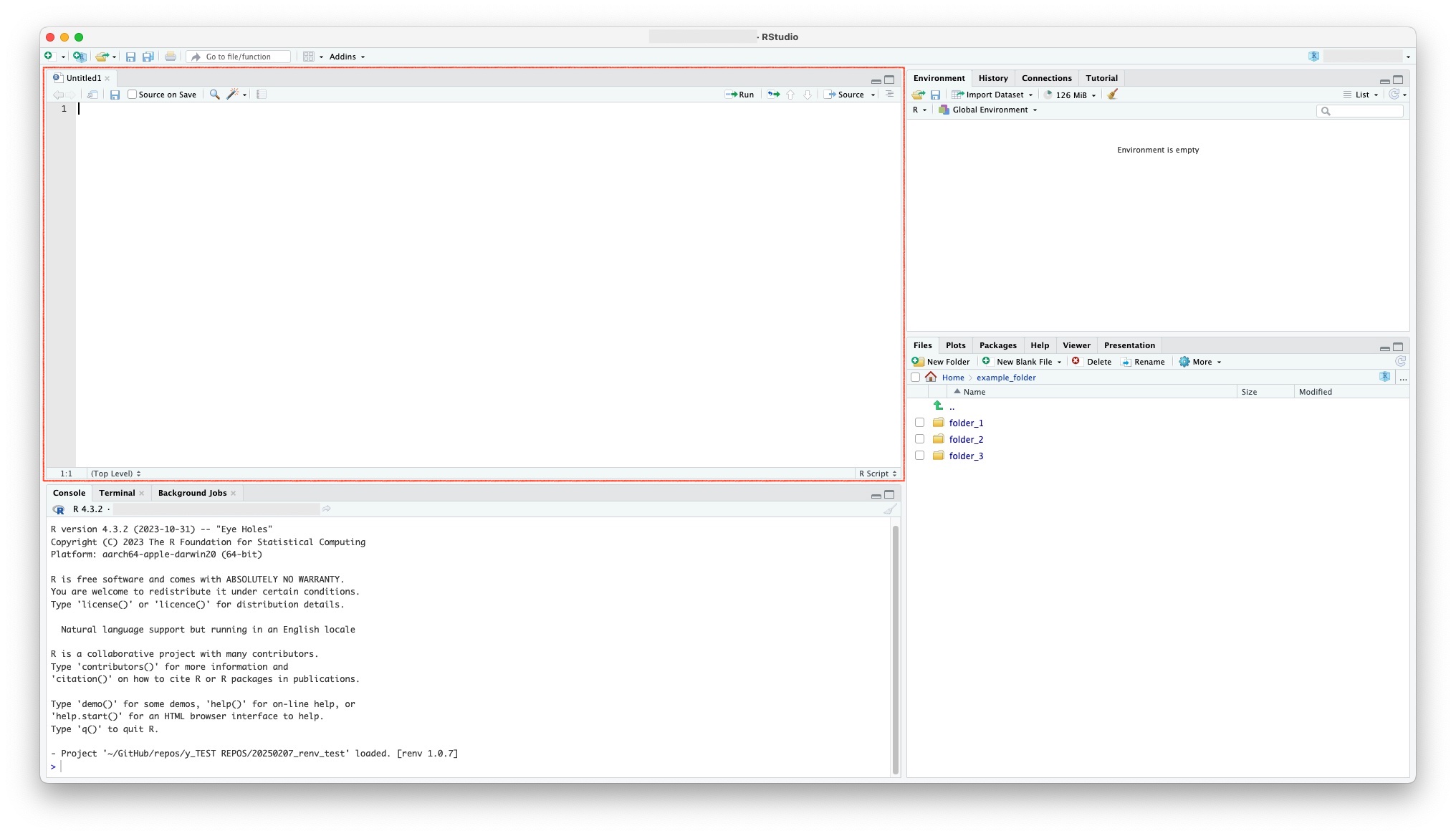
RStudio interface is built of a number of panels. It is too much to worry about what every tab in every section does, but the default tabs in the default 4 sections will do for now.
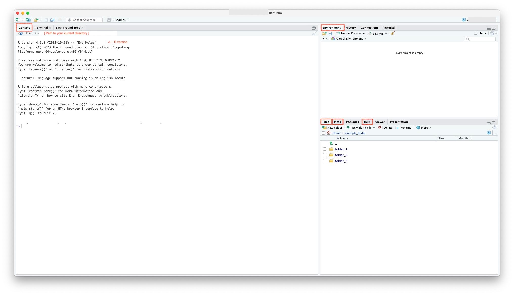
Left: Console: You can write code into the console section.
Top right: Environment pane: You will be able to see R objects you’ve created in this pane.
Bottom right: Files pane: Shows the folders + files architecture of your current folder (typically your User directory by default). Later on we’ll see that this pane can also show you your Plots and find Help documentation.
4.2 Using the Console
So how do we get started with running R commands? We can start in the console. This is the interactive section in which (typically short) commands can be typed or pasted in, and run, and the outputs will appear below the command. You can tell the difference between a command you wrote and the output, as commands begin with `> ’ and outputs do not. On my version of RStudio, commands are also in blue font, whereas outputs appear in black or orange.
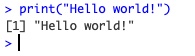
You can start by printing a message to the console with the following code:
To run this code, copy or type in the above text into your console, and press Enter.
A new line should appear with the printed text. What do you see?
It should be something like this:
What is the difference between the above and the following:
To run this code, copy or type in the above text into your console, and press Enter.
Typically, Warning and Error messages are printed as ‘messages’ in orange. Black text in the console is usually information you ask for from calculations or a print call.
You can also do basic arithmetic such as:
4.3 Assignments and Objects
Here is where the analogy with algebra ends. In R, we generally don’t use an = sign when we assign values to objects.
We use the assignment symbol, which is a left-pointing arrow <-.
While it is different from other coding languages that use =, R is actually clearer about what this line of code does. It does not represent an equivalence in a mathematical way, as we are not literally saying that x is the same as 10. Instead, when we write x <- 10, we are taking the value 10 and putting it into an object called x. We are “assigning” the value 10 to the object x.
In R, objects can be thought of as containers for values. In practice, they are a way of naming values as a shortcut to writing out the values again. In other words, the values that objects contain can later be called by using its name (see below for calling the value of x in different ways). An object can contain a numeric value like 10, but it could also contain a character or string value (a word or phrase) like “plasmid” or “strain” or “plot1.png”.
GLOSSARY: There is a glossary of terms in the Appendices if you want to later look up the definitions of words like object, character or string.
Notice that before we wrote the line x <- 10, calling x would have led to an error, because the object x didn’t exist. Now it does, and it contains the value 10.
You can witness this by calling the object y, which doesn’t yet exist:
Congratulations, you got your first error message! Happily, we don’t need to worry about this one.
Going back to x, notice that we can change the value of x at any time by writing another assignment:
Note that running code that assigns a value to x twice will NEVER create a second object called x. It will ALWAYS overwrite the first value given to x. This is one reason we always need to be careful that all our objects have unique names.
We can check the value of x in multiple ways. The basic would be to use the print function from above.
But there’s actually a shortcut. R allows you to simply put in the object name, and this will give you its value directly.
The Environment Tab will also tell you the current values of any assigned object. Have a look and see if you can find it.
4.4 The tidyverse
A package or library is a set of related R functions. A function is a ‘module’ of code written to accomplish a specific task. Common packages include ggplot2, which includes functions devoted to building various types of plots.
Run the following code to install the tidyverse packages.
This will install the packages we will need for data manipulation and visualisation for all 3 workshops. It includes ggplot, dplyr, tidyr, readr and stringr - though the package names don’t matter for the purposes of these workshops. This may take a few minutes, particularly if your R is new, as you may need some basic packages installed first before the tidyverse ones will function. You should see the progress in the Console as packages download. R will organise them carefully for quick loading later, so you don’t need to worry about any of that.
To test the tidyverse packages have installed correctly, we will need some example data. As it happens, there’s a nice data package that contains a set of data about Antarctic penguins that we can use for this purpose. Run the following to install it.
This package contains a dataset called penguins. We can view it by (a) loading the package, then (b) calling the dataset object’s name. (Copy/paste/run each line separately in the console.)
You should see the following in the console:
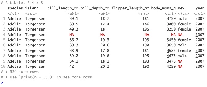
Notice what we’re doing when we run penguins is identical to running x above. We’re calling an object called penguins and asking to see what it contains. Unlike x above, it doesn’t just contain a single numerical value, but an entire data table. Data tables in R are called data frames. We will be working a lot with data frames!
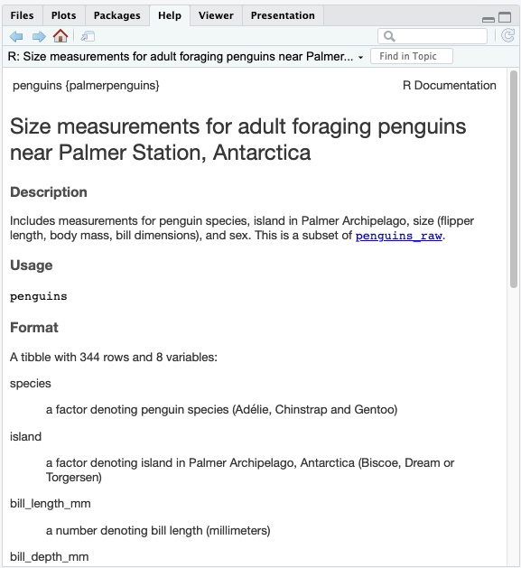
If you’d like more info on a dataset, use the notation ?dataset.
This should open the Help Tab in the bottom left to give you some information on the dataset, such as an explanation of the column names.
To test out tidyverse, let’s move from the console to the scripting pane. We’ll need more than single line code for this test.
4.5 Scripting
Create a new R file with File > New File > R script. You should see RStudio nudging the Console down to make room for your new script. While it might be easier to save your script for now, you don’t need to worry about where to save this script as you won’t need it again. We’ll talk more about how and where to save script files in Workshop 1.
R scripts allow us to write and execute code not just interactively, line by line, but to build up more complex scripts of 100s or even 1000s lines of code. Eventually, these can be run automatically, but to understand how our scripts work, we will run them line by line. This will help you see the effect of each line of code. Pay attention in the workshops to outputs of the code, which may appear in the Console, the Plots Tab and the Environment Tab.
Copy the following code and paste it into your script.
Run the code line by line by placing the cursor at the beginning or end of each line, and running that line with Cmd+Enter (on MacOS) or Ctrl+Enter (on Windows).
Notice that you can’t run the lines beginning #. The hash at the beginning of the line turns it into a comment that allows us to explain our script to others we share it with (or ourselves as a reminder). However, lines containing comments to the right are run: R reads from left to right until it hits a #. So we can add comments either on their own line, or to the RIGHT of R commands. You should see comments in green in RStudio if you set your editor to Crimson Red.
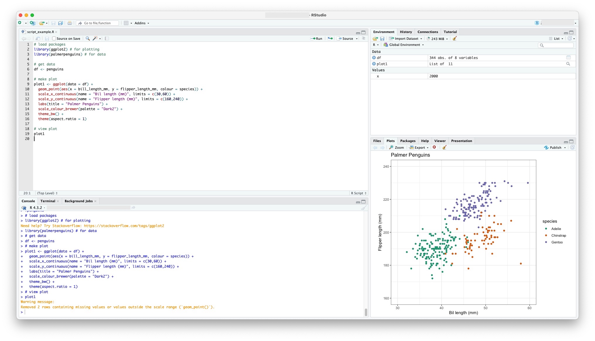
# load packages
library(ggplot2) # for plotting
library(palmerpenguins) # for data

# get data
df <- penguins

# make plot
plot1 <- ggplot(data = df) +
  geom_point(aes(x = bill_length_mm, y = flipper_length_mm, colour = species)) +
  scale_x_continuous(name = "Bill length (mm)", limits = c(30,60)) +
  scale_y_continuous(name = "Flipper length (mm)", limits = c(160,240)) +
  labs(title = "Palmer Penguins") +
  scale_colour_manual(values = c("#FF6C01", "#C65BCA", "#0F7075")) +
  theme_bw() +
  theme(aspect.ratio = 1)

# view plot
plot1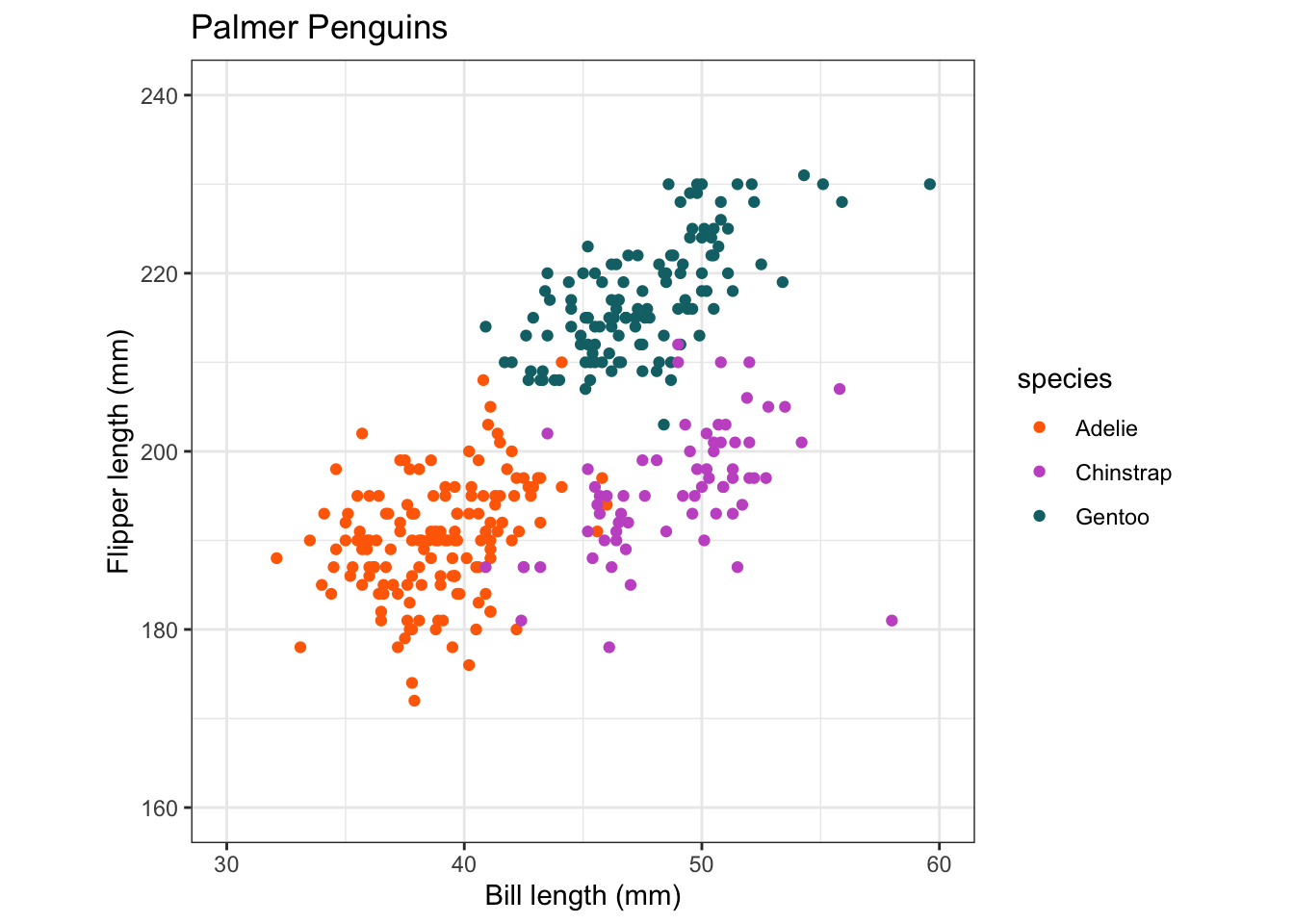
What does each line do?
library(ggplot2)loads one of the tidyverse libraries into the R session. Without loading the package, we would not be able to use its functions. To go back to the kitchen analogy, our tools would be installed (in the cupboard) but not on the kitchen counter, where we need them!The second line
df <- penguinsrenames thepenguinsdataset to call itdf, which is short for dataframe. While renaming objects is not usually necessary, it’s worth getting used to notation like dataframe and its short form df as they’re used ubiquitously in R as object names for data sets.The third line is a compound of 8 lines joined together by
+symbols that build up a plot layer by layer. We’ll go into the details in Workshop 1. This plot is assigned to an object calledplot1.The fourth line calls the
plot1object to view what it contains. When you run this line, you should see the above plot appear in your Plots tab.
The plot itself is unimportant here, as this is just a toy dataset: this data isn’t similar to the data we’ll be using later, it’s just for illustration.
This is what your RStudio should look like:
If you managed to reproduce the plot, congratulations! You are already plotting with R. And notice this can be done with very few lines of code. We will go into more detail about how to craft beautiful plots for biological datasets with R in Workshop 1.
4.6 A recap on objects
As stated above, objects are containers that can contain any value, whether numeric or a string (word like “plasmid”). What we didn’t specify above was that objects do not need to contain just a value. Notice that in the script above, we encountered two more types of object. Whereas x contained just a single numeric 10, the objects penguins and df contain an entire dataframe, and the object plot contains an entire plot!
A frequent cause of errors is when we write code that attempts to do something ‘illegal’ with the objects we provide as inputs. For instance, we cannot multiply a word like “plasmid”, and nor can we take the average of a plot. But it’s easy sometimes to write code that causes this type of error. Look out for errors that are caused by this kind of mistake.
4.7 Summary
- RStudio consists of 4 main panels.
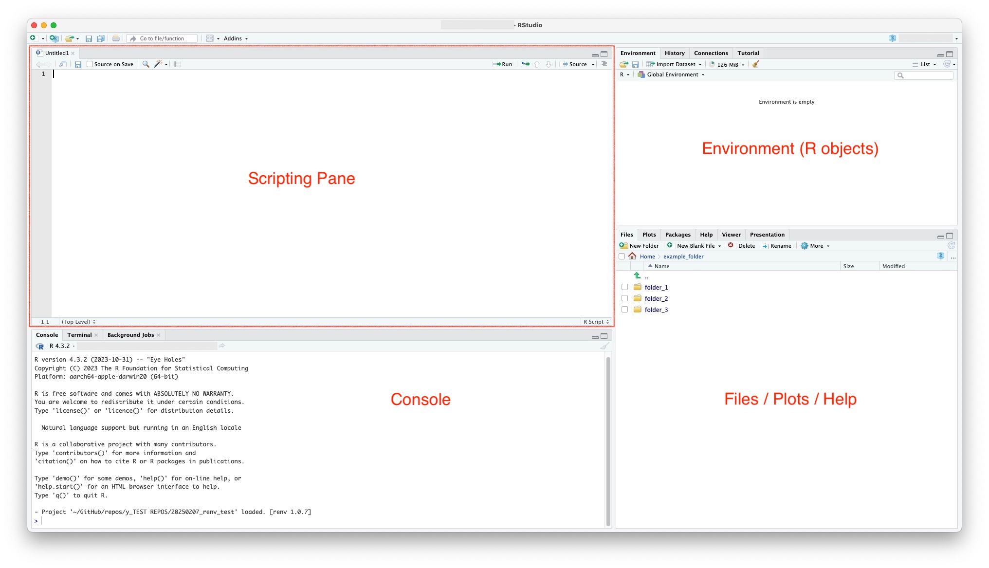
- Top left: Scripting pane: this is where your scripts will open, once you have some. (At the beginning, it may be minimised.)
- Bottom left: Console: this is where your code gets executed. Type it in directly, or execute code from your documents pane with the keyboard shortcut Crtl/Cmd + Enter.
- Top right: Environment pane: Visually explore all the R objects you’ve created.
- Bottom right: Files viewer, Plots viewer and Help sections.
Or if you prefer cake based metaphors:
We can run simple commands directly in the console.
To run more complex analyses, we write multi-line code into a script. Running this produces outputs in the console (dataframes and calculation outputs), Environment pane (saved objects), Plots tab (plots) and Help tab (documentation).
4.8 To check before proceeding
- Can you open RStudio and run basic arithmetic, basic assignment code in the console and reproduce expected outputs?
- Have you installed the tidyverse packages successfully?
- Can you reproduce the
penguinsdata plot?
If this all works for you, congrats, you’re done with the prep work for Workshop 1!