The first step in any data analysis workflow is converting raw data
produced by a data source (in our case, a plate reader) into a format
that may be manipulated effectively for analysis. The
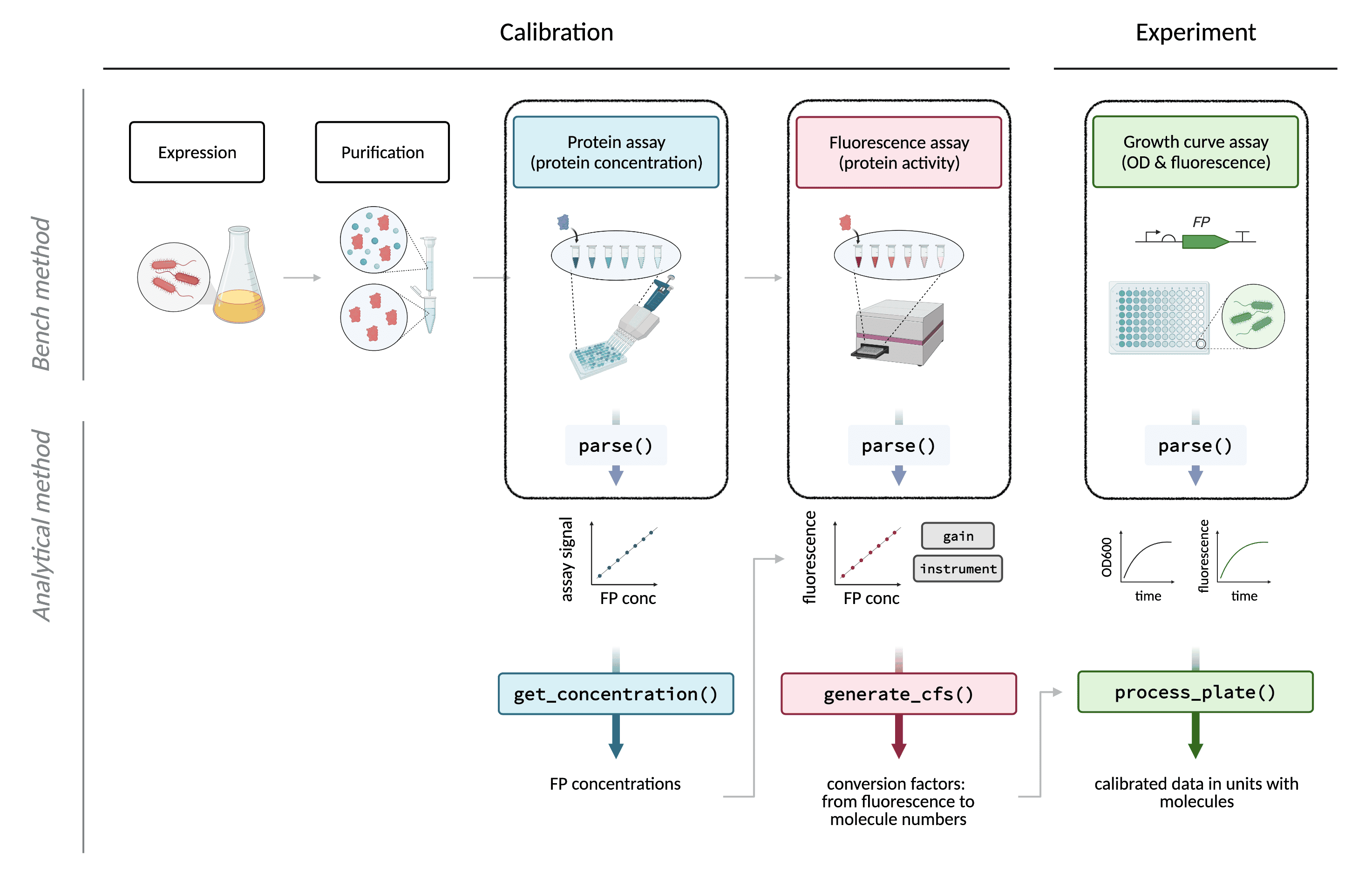
parse() symbols in the overview figure below indicate that
this is required for data output from each of the types of raw data
analysed by this package: the spectrum data from the absorbance assay,
the endpoint data from the fluorescence assay, and the
endpoint/timecourse data from the experimental assay.

Data parsing functions read raw data to: (1) extract data from the raw data file (removing unnecessary information), (2) tidy data into a so-called ‘tidy data’* format and (3) join data to appropriate metadata necessary for their analysis (such as information about the details of the samples in each well, the identity of the plate reader used, etc.).
*Tidy data is of the form where every column is a variable, every row is an observation, and every cell contains a single value.
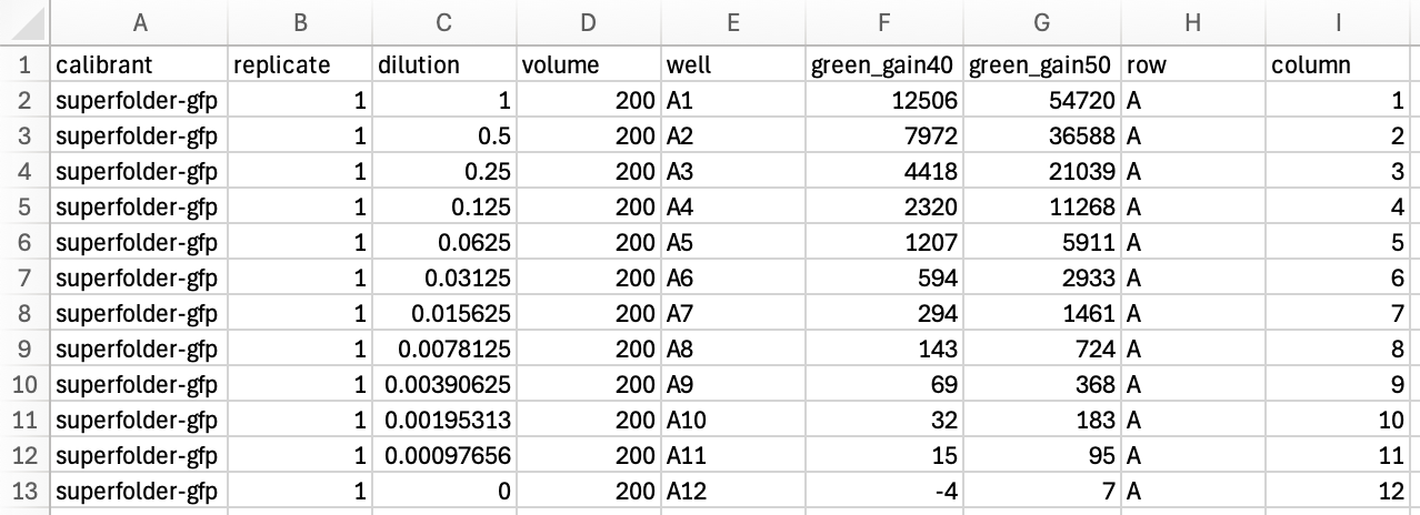
To appreciate what parsing does to data, consider the differences between the following raw data:

..and parsed data:

In order to parse your data, you will need to create a metadata file, and identify a parsing method for it.
Metadata Requirements
What do we mean by metadata and why is it necessary? Some metadata is
essential for calculations, such as the ability to group samples by a
variable, and take a mean or standard deviation for each level
(e.g. according to which dilution we measured in a
calibration, or the level of inducer_concentration that was
used in an experiment). Others are required to specify axes in plots,
e.g. dilution for calibrations or time for a
timecourse experiment. Still others are used to verify calculations:
calibration values will differ for different instruments, so
instrument is a crucial bit of metadata for every
calibration.
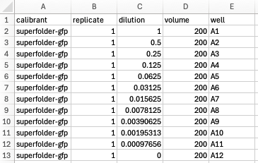
Metadata files should be prepared in ‘tidy data’ format, and may look something like this, although the exact variables will differ for each assay type.

For calibrations: absorbance spectra
| Function | Metadata Expected | Required For |
|---|---|---|
| parse_magellan_spectrum() | well | generating 'row' and 'column' variables |
| process_absorbance_spectrum() | instrument | reproducibility |
| plate | reproducibility | |
| seal | reproducibility | |
| media | reproducibility | |
| calibrant | checking number of calibrants | |
| protein | removing unused wells | |
| finding blank wells | ||
| dilution | separating plots | |
| identifying blanks | ||
| plotting as x axis | ||
| replicate | colouring plots | |
| volume | finding path lengths | |
| well | finding measurement columns | |
| path length calculations | ||
| row | finding measurement columns | |
| finding rows to keep | ||
| column | finding columns to keep | |
| get_conc_ecmax() | instrument | reproducibility |
| grouping | ||
| plate | reproducibility | |
| seal | reproducibility | |
| media | reproducibility | |
| grouping | ||
| calibrant | grouping | |
| protein | finding blank wells | |
| grouping | ||
| dilution | calculating concentration | |
| plotting | ||
| grouping | ||
| well | removing wells |
For calibrations: fluorescence data
| Function | Metadata Expected | Required For |
|---|---|---|
| parse_magellan() | well | generating 'row' and 'column' variables |
| generate_cfs() | instrument | reproducibility |
| plate | reproducibility | |
| seal | reproducibility | |
| channel_name | verifying cfs file matches channel used | |
| extracting gain | ||
| channel_ex | reproducibility | |
| channel_em | reproducibility | |
| media | reproducibility | |
| calibrant | verifying unique calibrants | |
| adding calibrant names to cfs files | ||
| protein | removing unused wells | |
| finding blank wells | ||
| mw_gmol1 | calculating molecule number | |
| concentration_ngul | calculating molecule number | |
| calculating dilution ratios | ||
| replicate | identifying saturated values | |
| volume | calculating molecule number | |
| well | finding measurement columns | |
| row | finding measurement columns |
For experimental data
| Function | Metadata Expected | Required For |
|---|---|---|
| parse_magellan() | well | generating 'row' and 'column' variables |
| process_plate() | volume | converting 'OD' to 'OD (cm-1)' |
| row | plotting data in 'microplate' format | |
| column | plotting data in 'microplate' format |
Notes:
- Variables that are not required for calculations are included for the sake of reproducibility.
-
channel_name/ex/emrefers to the fluorescence ‘channel’, i.e. filter set. The one most commonly used for GFPs includes excitation filter at 485nm with 20nm bandwidth and emission at 535nm with 25nm bandwidth. For this,channel_namemay be ‘green’ or ‘blue_ex_green_em’ or anything that is concise and meaningful for your calibrations. If you are taking calibrations at several gains (as is recommended), the names given to your fluorescence measurements/readings must match the value inchannel_nameexactly (e.g.channel_name= ‘green’ and measurements taken are called ‘green_40’, ‘green_50’, .. ‘green_120’).channel_excould be “485/20”. -
proteinis expected to equal “none” for the blank/buffer wells and to be empty for wells that were not used in the assay. -
dilutionshould be specified as 1 for the undiluted sample, 0.5 for a 2-fold diluted sample, etc.dilutionmust be left blank for blank and buffer wells. -
mw_gmol1is molecular weight in g/mol. -
concentration_ngulis concentration in ng/ul. -
rowandcolumnare also expected in every function above, but these should be auto-generated by the parser function from the metadatawellcolumn. -
timeshould be auto-generated by the parser function for timecourse data.
Save metadata templates
For a shortcut to creating your own metadata templates, run:
save_metadata_template(
  data_type = "absspectrum", # OPTIONS: "absspectrum", "fluordata", "exptdata"
  plate_type = 96, # 96 for 96-well plate, etc
  outfolder = "templates" # where to save files
)
Methods for Parsing Data
Using Tecan Spark plate readers
As fpcountr was developed in a laboratory that used
Tecan Spark instruments, we have bundled functions into the package that
can parse data exported from Spark plate readers. You will need
different parsing functions depending on whether you are using their
Magellan software or their SparkControl software.
Magellan software parsers
parse_magellan() handles standard/endpoint and
timecourse/kinetic data. To parse a data file, the minimum information
you need is the location of your data and metadata files, and
whether/not your data is a timeseries (i.e. timecourse/kinetic data).
For fluorescence data from endpoint/standard assays, such as
calibrations, you might use:
parsed_data <- parse_magellan(
  data_csv = "path/to/data.csv",
  metadata_csv = "path/to/metadata.csv",
  timeseries = FALSE,
  save_file = TRUE
)
This function can work out the number of readings with no extra
information, assuming that the only exported information is data, and
not metadata. If the raw data export file includes lines above and below
the fluorescence or absorbance data occupied by metadata such as ‘Well
Positions’, ‘Layout’ or ‘Replicate Info’, this needs indicating with
metadata_above (to indicate lines above the data taken up
by such metadata), or metadata_below.
parsed_data <- parse_magellan(
  data_csv = "path/to/data.csv",
  metadata_csv = "path/to/metadata.csv",
  timeseries = FALSE,
  metadata_above = 1,
  metadata_below = 0,
  save_file = TRUE
)
Further, if you exported temperature data with the fluorescence data,
causing the data to be right-shifted from the otherwise default second
column, use custom = TRUE and specify startcol
and endcol.
parsed_data <- parse_magellan(
  data_csv = "path/to/data.csv",
  metadata_csv = "path/to/metadata.csv",
  timeseries = FALSE,
  custom = TRUE, startcol = 3, endcol = 98,
  save_file = TRUE
)
If the data does not include all 96 wells expected, e.g. it is
truncated at H11 instead of H12 due to export options, you can use
insert_wells_below = 1 which will add a blank line at the
end of the data. This can help with matching metadata files containing
entries for 96 wells with data containing fewer than 96 entries.
parsed_data <- parse_magellan(
  data_csv = "path/to/data.csv",
  metadata_csv = "path/to/metadata.csv",
  timeseries = FALSE,
  custom = TRUE,
  startcol = 3,
  endcol = 97,
  insert_wells_above = 0,
  insert_wells_below = 1,
  save_file = TRUE
)
For timecourse/kinetic assays, such as from microbial growth curve
experiments, choose timeseries = TRUE and specify:
-
timestart: the text in column 1 with which to identify the first row of data. This is usually “0s”. -
interval: the number of minutes between any 2 readings -
mode: which specifies whether an interval starts with readings (“read_first”) or an incubation (“incubate_first”). This will normally be “read_first”.
parsed_data <- parse_magellan(
  data_csv = "path/to/data.csv",
  metadata_csv = "path/to/metadata.csv",
  timeseries = TRUE,
  timestart = "0s",
  interval = 10, # in minutes
  mode = "read_first", # mode can only be "read_first" or "incubate_first"
  metadata_above = 1,
  metadata_below = 0,
  custom = TRUE,
  startcol = 3,
  endcol = 97,
  insert_wells_above = 0,
  insert_wells_below = 1,
  save_file = TRUE
)
A separate function, parse_magellan_spectrum(), should
be used to parse spectrum data. It works similarly.
parsed_data_spectrum <- parse_magellan_spectrum(
  data_csv = "path/to/data.csv",
  metadata_csv = "path/to/metadata.csv",
  wellstart = "A1", wellend = "H12",
  save_file = TRUE
)
It is worth sanity checking outputs to make sure that the data has been extracted correctly, and adjusting the customisation parameters if it isn’t.
SparkControl software parsers
Analogous functions exist also for the SparkControl software exports.
parse_sparkcontrol() handles standard/endpoint and
timecourse/kinetic data:
parsed_data <- parse_sparkcontrol(
  data_csv = "path/to/data.csv",
  metadata_csv = "path/to/metadata.csv",
  timeseries = FALSE,
  save_file = TRUE
)

parsed_data <- parse_sparkcontrol(
  data_csv = "path/to/data.csv",
  metadata_csv = "path/to/metadata.csv",
  timeseries = TRUE,
  save_file = TRUE
)
and parse_sparkcontrol_spectrum() handles spectrum
data:
parsed_data_spectrum <- parse_sparkcontrol_spectrum(
  data_csv = "path/to/data.csv",
  metadata_csv = "path/to/metadata.csv",
  wellstart = "A1", wellend = "H12",
  save_file = TRUE
)
Examples
1. Absorbance spectrum data for a calibration of mTagBFP2
Raw data:
| V1 | V2 | V3 | V4 | V5 | V6 | V7 | V8 | V9 | V10 | V11 |
|---|---|---|---|---|---|---|---|---|---|---|
| Spectrum data | NA | NA | NA | NA | NA | NA | NA | NA | NA | |
| [nm] | 200.0000 | 201.0000 | 202.0000 | 203.0000 | 204.0000 | 205.0000 | 206.0000 | 207.0000 | 208 | 209.0000 |
| A1 | 3.2934 | 3.2799 | 3.3390 | 3.3396 | 3.3812 | 3.3875 | 3.4014 | 3.3519 | 3.3743 | 3.3190 |
| B1 | 3.2622 | 3.3121 | 3.3903 | 3.6836 | 3.4257 | 3.3808 | 3.4499 | 3.4804 | 3.4558 | 3.3016 |
| A2 | 3.2612 | 3.3153 | 3.3262 | 3.3553 | 3.4475 | 3.3497 | 3.3685 | 3.3631 | 3.389 | 3.3843 |
| B2 | 3.2615 | 3.2786 | 3.3289 | 3.5397 | 3.4848 | 3.3831 | 3.4237 | 3.4103 | 3.4671 | 3.3550 |
| A3 | 3.2943 | 3.3587 | 3.3668 | 3.3376 | 3.3925 | 3.3521 | 3.3763 | 3.3388 | 3.3662 | 3.3503 |
| B3 | 3.2896 | 3.3469 | 3.3185 | 3.3641 | 3.3797 | 3.2989 | 3.3664 | 3.3426 | 3.3452 | 3.3142 |
| A4 | 3.2608 | 3.3900 | 3.3016 | 3.3737 | 3.4401 | 3.3511 | 3.4485 | 3.3411 | 3.5792 | 3.4078 |
Code:
parsed_data <- parse_magellan_spectrum(
  data_csv = "data/example_absorbance.csv",
  metadata_csv = "data/example_absorbance_meta.csv",
  wellstart = "A1", wellend = "B12",
  save_file = TRUE
)
## 24 wells identified.Parsed data:
| instrument | calibrant | dilution | well | 200 | 201 | 202 | 203 | 204 | 205 | 206 | 207 | 208 |
|---|---|---|---|---|---|---|---|---|---|---|---|---|
| spark1 | mTagBFP2 | 1.000000000 | A1 | 3.2934 | 3.2799 | 3.3390 | 3.3396 | 3.3812 | 3.3875 | 3.4014 | 3.3519 | 3.3743 |
| spark1 | mTagBFP2 | 0.500000000 | A2 | 3.2612 | 3.3153 | 3.3262 | 3.3553 | 3.4475 | 3.3497 | 3.3685 | 3.3631 | 3.3890 |
| spark1 | mTagBFP2 | 0.250000000 | A3 | 3.2943 | 3.3587 | 3.3668 | 3.3376 | 3.3925 | 3.3521 | 3.3763 | 3.3388 | 3.3662 |
| spark1 | mTagBFP2 | 0.125000000 | A4 | 3.2608 | 3.3900 | 3.3016 | 3.3737 | 3.4401 | 3.3511 | 3.4485 | 3.3411 | 3.5792 |
| spark1 | mTagBFP2 | 0.062500000 | A5 | 3.2948 | 3.3343 | 3.3076 | 3.5574 | 3.7229 | 3.8790 | 3.4160 | 3.3230 | 3.8098 |
| spark1 | mTagBFP2 | 0.031250000 | A6 | 3.2894 | 3.3136 | 3.3454 | 3.4588 | 3.3556 | 3.3564 | 3.3910 | 3.4368 | 3.2939 |
| spark1 | mTagBFP2 | 0.015625000 | A7 | 3.2930 | 3.3226 | 3.3383 | 3.3680 | 3.3786 | 3.4243 | 3.4188 | 3.2832 | 3.3297 |
| spark1 | mTagBFP2 | 0.007812500 | A8 | 3.2936 | 3.3589 | 3.3350 | 3.3625 | 3.4282 | 3.3435 | 3.3975 | 3.3195 | 3.4037 |
| spark1 | mTagBFP2 | 0.003906250 | A9 | 3.2909 | 3.2733 | 3.3648 | 3.3259 | 3.4149 | 3.3244 | 3.4223 | 3.3273 | 3.3610 |
| spark1 | mTagBFP2 | 0.001953125 | A10 | 3.2934 | 3.2913 | 3.3022 | 3.4590 | 3.4969 | 3.3739 | 3.3996 | 3.4085 | 3.3520 |
| spark1 | mTagBFP2 | 0.000976563 | A11 | 3.2608 | 3.2641 | 3.3324 | 3.3941 | 3.4011 | 3.3272 | 3.4094 | 3.3708 | 3.3890 |
| spark1 | mTagBFP2 | NA | A12 | 3.2570 | 3.3090 | 3.3415 | 3.3510 | 3.3476 | 3.3447 | 3.4181 | 3.3793 | 3.3385 |
2. Fluorescence data for a calibration of mTagBFP2
Raw data:
| V1 | V2 | V3 | V4 | V5 | V6 | V7 | V8 | V9 | V10 | V11 | V12 | V13 | V14 | V15 | V16 | V17 | V18 |
|---|---|---|---|---|---|---|---|---|---|---|---|---|---|---|---|---|---|
| blueblue040 | NA | NA | NA | NA | NA | NA | NA | NA | NA | ||||||||
| blueblue050 | NA | NA | NA | NA | NA | NA | NA | NA | NA | ||||||||
| blueblue060 | NA | NA | NA | NA | NA | NA | NA | NA | NA | ||||||||
| blueblue070 | NA | NA | NA | NA | NA | NA | NA | NA | NA | ||||||||
| blueblue080 | NA | NA | NA | NA | NA | NA | NA | NA | NA | ||||||||
| blueblue090 | NA | NA | NA | NA | NA | NA | NA | NA | NA | ||||||||
| blueblue100 | NA | NA | NA | NA | NA | NA | NA | NA | NA | ||||||||
| blueblue110 | NA | NA | NA | NA | NA | NA | NA | NA | NA | ||||||||
| blueblue120 | NA | NA | NA | NA | NA | NA | NA | NA | NA | ||||||||
| 0s | 133 | 68 | 36 | 19 | 11 | 7 | 4 | 4 | 3 | 3 | 3 | 3 | 134 | 74 | 35 | 19 | 11 |
| 43s | 737 | 394 | 219 | 131 | 88 | 65 | 54 | 49 | 46 | 45 | 45 | 43 | 751 | 431 | 219 | 132 | 93 |
| 80s | 2960 | 1588 | 886 | 540 | 370 | 278 | 233 | 213 | 200 | 198 | 194 | 191 | 2986 | 1720 | 889 | 546 | 385 |
| 118s | 9097 | 4875 | 2739 | 1662 | 1153 | 861 | 730 | 663 | 631 | 625 | 608 | 595 | 9180 | 5292 | 2718 | 1676 | 1199 |
Code:
parsed_data <- parse_magellan(
  data_csv = "data/example_fluorescence.csv",
  metadata_csv = "data/example_fluorescence_meta.csv",
  timeseries = FALSE,
  custom = TRUE,
  startcol = 2,
  endcol = 25,
  insert_wells_above = 0,
  insert_wells_below = 72,
  save_file = TRUE
)
Parsed data:
| instrument | channel_name | channel_ex | channel_em | calibrant | well | blueblue040 | blueblue050 | blueblue060 | blueblue070 | blueblue080 | blueblue090 | blueblue100 | blueblue110 | blueblue120 |
|---|---|---|---|---|---|---|---|---|---|---|---|---|---|---|
| spark1 | blueblue | 400/20 | 465/35 | mTagBFP2 | A1 | 133 | 737 | 2960 | 9097 | 22595 | 50522 | NA | NA | NA |
| spark1 | blueblue | 400/20 | 465/35 | mTagBFP2 | A2 | 68 | 394 | 1588 | 4875 | 12140 | 27526 | 57864 | NA | NA |
| spark1 | blueblue | 400/20 | 465/35 | mTagBFP2 | A3 | 36 | 219 | 886 | 2739 | 6849 | 15485 | 32882 | 64351 | NA |
| spark1 | blueblue | 400/20 | 465/35 | mTagBFP2 | A4 | 19 | 131 | 540 | 1662 | 4154 | 9504 | 20037 | 39740 | NA |
| spark1 | blueblue | 400/20 | 465/35 | mTagBFP2 | A5 | 11 | 88 | 370 | 1153 | 2868 | 6530 | 13895 | 27655 | 51126 |
| spark1 | blueblue | 400/20 | 465/35 | mTagBFP2 | A6 | 7 | 65 | 278 | 861 | 2168 | 4945 | 10525 | 20781 | 38599 |
| spark1 | blueblue | 400/20 | 465/35 | mTagBFP2 | A7 | 4 | 54 | 233 | 730 | 1830 | 4166 | 8822 | 17547 | 32679 |
| spark1 | blueblue | 400/20 | 465/35 | mTagBFP2 | A8 | 4 | 49 | 213 | 663 | 1668 | 3787 | 8036 | 15969 | 29849 |
| spark1 | blueblue | 400/20 | 465/35 | mTagBFP2 | A9 | 3 | 46 | 200 | 631 | 1582 | 3604 | 7658 | 15187 | 28256 |
| spark1 | blueblue | 400/20 | 465/35 | mTagBFP2 | A10 | 3 | 45 | 198 | 625 | 1555 | 3547 | 7516 | 14953 | 27956 |
| spark1 | blueblue | 400/20 | 465/35 | mTagBFP2 | A11 | 3 | 45 | 194 | 608 | 1523 | 3502 | 7404 | 14721 | 27357 |
| spark1 | blueblue | 400/20 | 465/35 | mTagBFP2 | A12 | 3 | 43 | 191 | 595 | 1504 | 3400 | 7237 | 14436 | 26968 |
3. Experimental data
Raw data:
| V1 | V2 | V3 | V4 | V5 | V6 | V7 | V8 | V9 | V10 | V11 | V12 | V13 | V14 | V15 | V16 |
|---|---|---|---|---|---|---|---|---|---|---|---|---|---|---|---|
| Well positions | NA | NA | NA | ||||||||||||
| OD600 | NA | NA | NA | ||||||||||||
| OD700 | NA | NA | NA | ||||||||||||
| blue | NA | NA | NA | ||||||||||||
| bluelow | NA | NA | NA | ||||||||||||
| NA | A2 | A3 | A4 | A5 | A6 | A7 | A8 | A9 | A10 | A11 | NA | NA | B2 | ||
| 0s | 30.2 °C | NA | 0.1255 | 0.1276 | 0.1323 | 0.1219 | 0.1294 | 0.129 | 0.1282 | 0.1228 | 0.1284 | 0.0969 | NA | NA | 0.1283 |
| 599s | 29.9 °C | NA | 0.1298 | 0.1318 | 0.1351 | 0.1244 | 0.1293 | 0.1297 | 0.1287 | 0.1216 | 0.1256 | 0.095 | NA | NA | 0.1281 |
| 1199s | 29.9 °C | NA | 0.1333 | 0.1355 | 0.1384 | 0.1272 | 0.1325 | 0.1323 | 0.1315 | 0.1246 | 0.1279 | 0.0942 | NA | NA | 0.1307 |
| 1799s | 29.9 °C | NA | 0.1383 | 0.1407 | 0.1436 | 0.131 | 0.1363 | 0.1359 | 0.1347 | 0.1278 | 0.1311 | 0.0937 | NA | NA | 0.1342 |
| 2399s | 29.8 °C | NA | 0.1429 | 0.1454 | 0.1484 | 0.1357 | 0.1409 | 0.1402 | 0.1391 | 0.1319 | 0.1348 | 0.0935 | NA | NA | 0.1388 |
Code:
parsed_data <- parse_magellan(
  data_csv = "data/example_experiment.csv",
  metadata_csv = "data/example_experiment_meta.csv",
  timeseries = TRUE,
  timestart = "0s",
  interval = 10, # minutes.
  mode = "read_first", # mode can only be "read_first" or "incubate_first"
  metadata_above = 1,
  metadata_below = 0,
  custom = TRUE,
  startcol = 3,
  endcol = 97,
  insert_wells_above = 0,
  insert_wells_below = 1,
  save_file = TRUE
)
Parsed data:
| media | strain | plasmid | inducer | ara_pc | volume | well | time | OD600 | OD700 | blue | bluelow |
|---|---|---|---|---|---|---|---|---|---|---|---|
| NA | A1 | 0 | NA | NA | NA | NA | |||||
| M9 | DH10B | pS361 | ara | 0 | 200 | A2 | 0 | 0.1255 | 0.1137 | 471 | 17 |
| M9 | DH10B | pS361 | ara | 0 | 200 | A3 | 0 | 0.1276 | 0.1121 | 472 | 17 |
| M9 | DH10B | pS361 | ara | 0 | 200 | A4 | 0 | 0.1323 | 0.1173 | 481 | 18 |
| M9 | DH10B | pS361 | ara | 0.3 | 200 | A5 | 0 | 0.1219 | 0.1088 | 479 | 17 |
| M9 | DH10B | pS361 | ara | 0.3 | 200 | A6 | 0 | 0.1294 | 0.1154 | 475 | 17 |
| M9 | DH10B | pS361 | ara | 0.3 | 200 | A7 | 0 | 0.1290 | 0.1152 | 472 | 17 |
| M9 | DH10B | pS361_ara_mTagBFP2 | ara | 0 | 200 | A8 | 0 | 0.1282 | 0.1139 | 468 | 17 |
| M9 | DH10B | pS361_ara_mTagBFP2 | ara | 0 | 200 | A9 | 0 | 0.1228 | 0.1090 | 466 | 17 |
| M9 | DH10B | pS361_ara_mTagBFP2 | ara | 0 | 200 | A10 | 0 | 0.1284 | 0.1144 | 469 | 17 |
| M9 | none | none | none | none | 200 | A11 | 0 | 0.0969 | 0.0910 | 473 | 17 |
| NA | A12 | 0 | NA | NA | NA | NA |
Using other plate readers
The above functions use clues from the Tecan Spark software’s standardised data formats to extract the data from raw files correctly, and therefore will not work for data from other plate readers.
For other plate readers, we recommend two options:
Writing your own functions
For more advanced users or when working with a large number of similar data files, writing your own functions will be the best option to automate parsing of a large number of files. Note that:
- the output needs to be ‘tidy data’
-
fpcountrfunctions additionally expect that the metadata is joined to the left of the data, and that thewellcolumn of the metadata has been used to create two further columns:row, andcolumn, which are placed to the right of the data. The resultant structure of required parsed data files are, left to right: [all metadata columns], [all data columns], ‘row’, ‘column’.
Using Parsley
For users who do not have time to do this or do not need to automate parsing, our recommended route is to use Parsley. Parsley is a web app we developed to allow you to parse data of any type into ‘tidy data’ format. The graphical user interface (GUI) lets you select the location of the data and all its characteristics within your raw data file using a point and click interface, and generates both a parsed data spreadsheet for you, as well as a ‘parser function’ file, that can be reused for parsing multiple data files. The software is free, available on the web and does not require the download of any software or the creation of any account. (However, you can install it from Github and run it locally if you would like to. Running it locally speeds it up.)
