Experiments II: Endpoint Cellular Fluorescence
Source:vignettes/expts_ii_endpoint.Rmd
expts_ii_endpoint.Rmd
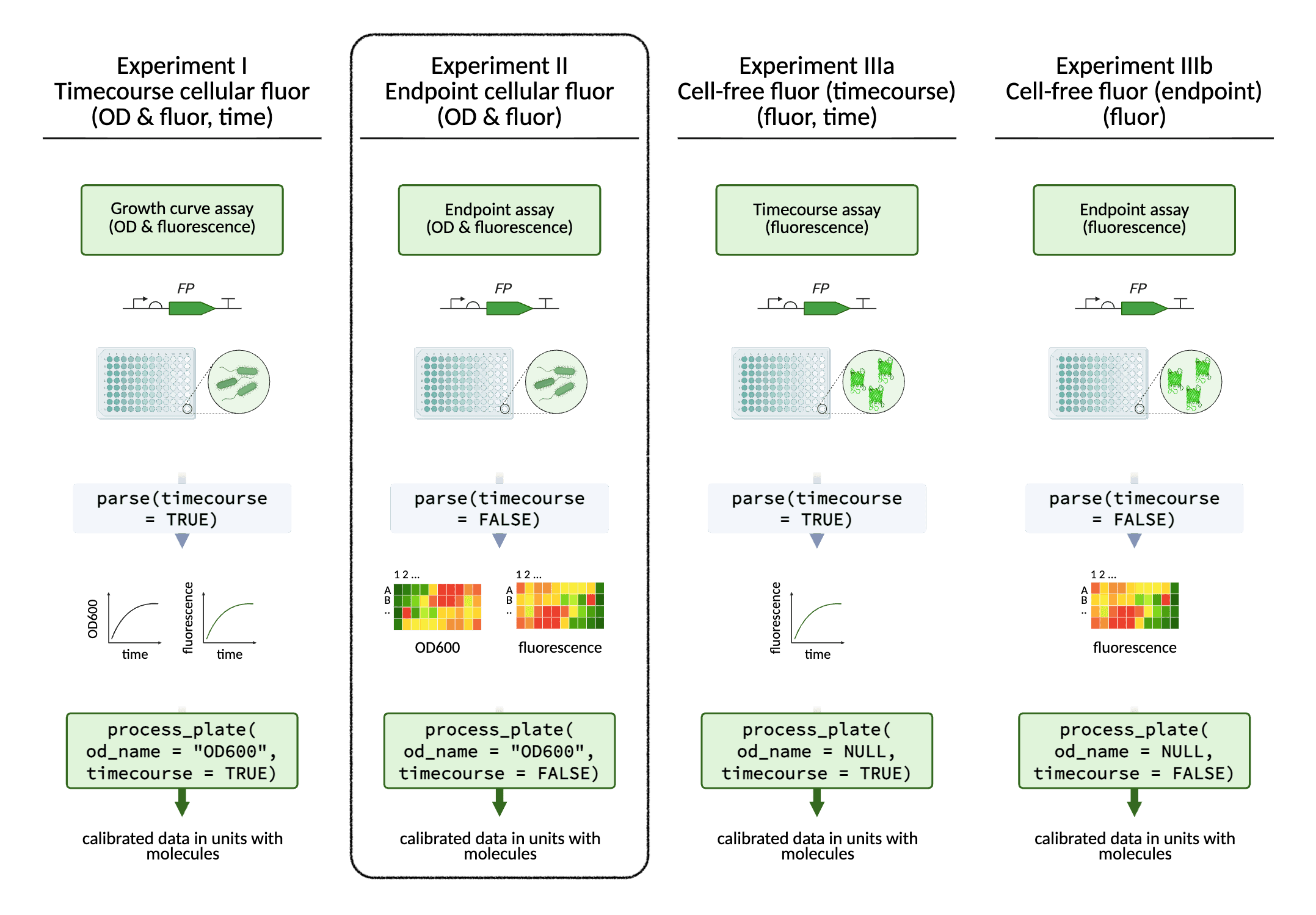
In addition to timecourse data, single timepoint fluorescence data
can also be processed with FPCountR, using the same functions. Just
apply the argument timecourse = FALSE.
Processing data from E. coli fluorescent protein expression experiments - single timepoint data
Example for single-timepoint data
Let’s consider an example in which cells expressing mTagBFP2 were grown in an incubator and transferred to the plate reader for a single timepoint scan. This data has already been parsed. With conversion factors for calibrating both mTagBFP2 fluorescence and cell number (OD) in hand, we are ready to process the experimental data.
parsed_data <- read.csv("data/example_experiment2_parsed.csv")
parsed_data[1:24,c(3,6:10)] # view a fragment of the dataframe| plasmid | ara_pc | volume | well | OD700 | blue |
|---|---|---|---|---|---|
| NA | A1 | NA | NA | ||
| pS361 | 0 | 200 | A2 | 0.5914 | 438 |
| pS361 | 0 | 200 | A3 | 0.5961 | 439 |
| pS361 | 0 | 200 | A4 | 0.6014 | 452 |
| pS361 | 0.3 | 200 | A5 | 0.6003 | 442 |
| pS361 | 0.3 | 200 | A6 | 0.5996 | 443 |
| pS361 | 0.3 | 200 | A7 | 0.6000 | 442 |
| pS361_ara_mTagBFP2 | 0 | 200 | A8 | 0.6001 | 441 |
| pS361_ara_mTagBFP2 | 0 | 200 | A9 | 0.5928 | 437 |
| pS361_ara_mTagBFP2 | 0 | 200 | A10 | 0.5911 | 438 |
| none | none | 200 | A11 | 0.0876 | 483 |
| NA | A12 | NA | NA | ||
| NA | B1 | NA | NA | ||
| pS361_ara_mTagBFP2 | 0.00003 | 200 | B2 | 0.6107 | 1297 |
| pS361_ara_mTagBFP2 | 0.00003 | 200 | B3 | 0.6017 | 1316 |
| pS361_ara_mTagBFP2 | 0.00003 | 200 | B4 | 0.6078 | 1337 |
| pS361_ara_mTagBFP2 | 0.0001 | 200 | B5 | 0.6108 | 2474 |
| pS361_ara_mTagBFP2 | 0.0001 | 200 | B6 | 0.6051 | 2363 |
| pS361_ara_mTagBFP2 | 0.0001 | 200 | B7 | 0.6054 | 2471 |
| pS361_ara_mTagBFP2 | 0.0003 | 200 | B8 | 0.5846 | 3270 |
| pS361_ara_mTagBFP2 | 0.0003 | 200 | B9 | 0.5808 | 3546 |
| pS361_ara_mTagBFP2 | 0.0003 | 200 | B10 | 0.5729 | 3458 |
| none | none | 200 | B11 | 0.0856 | 480 |
| NA | B12 | NA | NA |
Process data
Process the experimental data using process_plate().
processed_data <- process_plate(
  data_csv = "data/example_experiment2_parsed.csv",
  blank_well = c("A11", "B11", "C11", "D11", "E11", "F11", "G11", "H11"),

  # timecourse
  timecourse = FALSE, ### Note requirement to declare `timecourse = FALSE`

  # od
  od_name = "OD700",

  # fluorescence labels
  flu_channels = c("blue"),
  flu_channels_rename = c("blueblue"),

  # correction
  do_quench_correction = TRUE,
  od_type = "OD700",

  # calibrations
  do_calibrate = TRUE,
  instr = "spark1",
  flu_slugs = c("mTagBFP2"),
  flu_gains = c(60),
  flu_labels = c("mTagBFP2"),

  # conversion factors
  od_coeffs_csv = "conversion_factors/od_conversion_factors_assembled.csv",
  fluor_coeffs_csv = "conversion_factors/fp_conversion_factors_assembled.csv",

  # background autofluorescence subtraction
  af_model = NULL, ### Note this is a requirement for `timecourse = FALSE`

  outfolder = "experiment_analysis"
)
The arguments are described in the ‘Get Started’ vignette. The output CSV is similar.
The following differences apply for process_plate()
where timecourse = FALSE:
- No requirement for a column labelled
time. - Plots are in heatmap format, rather than line plot format.
- Autofluorescence correction cannot be carried out by any of the
model options, such as
splineorloess, because there isn’t enough data to do this. In practice, this means theaf_modelparameter is rewritten toNULL, and fluorescence normalisation takes place by simply subtracting the fluorescence of the blank wells.
processed_data[14:24,c(3,6,8,14:20)] # view a fragment of the dataframe| plasmid | ara_pc | well | pathlength | normalised_OD_cm1 | normalised_blueblue | flu_quench | corrected_normalised_blueblue | calibrated_OD | calibrated_mTagBFP2 |
|---|---|---|---|---|---|---|---|---|---|
| pS361_ara_mTagBFP2 | 0.00003 | B2 | 0.6072014 | 0.863593213 | 818.25 | 0.7888225 | 1037.305602 | 527056389.0 | 1.143966e+13 |
| pS361_ara_mTagBFP2 | 0.00003 | B3 | 0.6072014 | 0.848771113 | 837.25 | 0.7908680 | 1058.646922 | 518010367.5 | 1.167502e+13 |
| pS361_ara_mTagBFP2 | 0.00003 | B4 | 0.6072014 | 0.858817203 | 858.25 | 0.7894782 | 1087.110453 | 524141559.8 | 1.198892e+13 |
| pS361_ara_mTagBFP2 | 0.0001 | B5 | 0.6072014 | 0.863757903 | 1995.25 | 0.7887999 | 2529.475317 | 527156900.3 | 2.789567e+13 |
| pS361_ara_mTagBFP2 | 0.0001 | B6 | 0.6072014 | 0.854370573 | 1884.25 | 0.7900916 | 2384.850104 | 521427753.4 | 2.630071e+13 |
| pS361_ara_mTagBFP2 | 0.0001 | B7 | 0.6072014 | 0.854864643 | 1992.25 | 0.7900233 | 2521.761093 | 521729287.4 | 2.781060e+13 |
| pS361_ara_mTagBFP2 | 0.0003 | B8 | 0.6072014 | 0.820609122 | 2791.25 | 0.7948423 | 3511.702973 | 500822926.8 | 3.872792e+13 |
| pS361_ara_mTagBFP2 | 0.0003 | B9 | 0.6072014 | 0.814350902 | 3067.25 | 0.7957414 | 3854.581279 | 497003495.5 | 4.250926e+13 |
| pS361_ara_mTagBFP2 | 0.0003 | B10 | 0.6072014 | 0.801340391 | 2979.25 | 0.7976297 | 3735.129191 | 489063098.9 | 4.119192e+13 |
| none | none | B11 | 0.6072014 | -0.001194003 | 1.25 | 0.9929566 | 1.258867 | -728707.3 | 1.388309e+10 |
| B12 | NA | NA | NA | NA | NA | NA | NA |
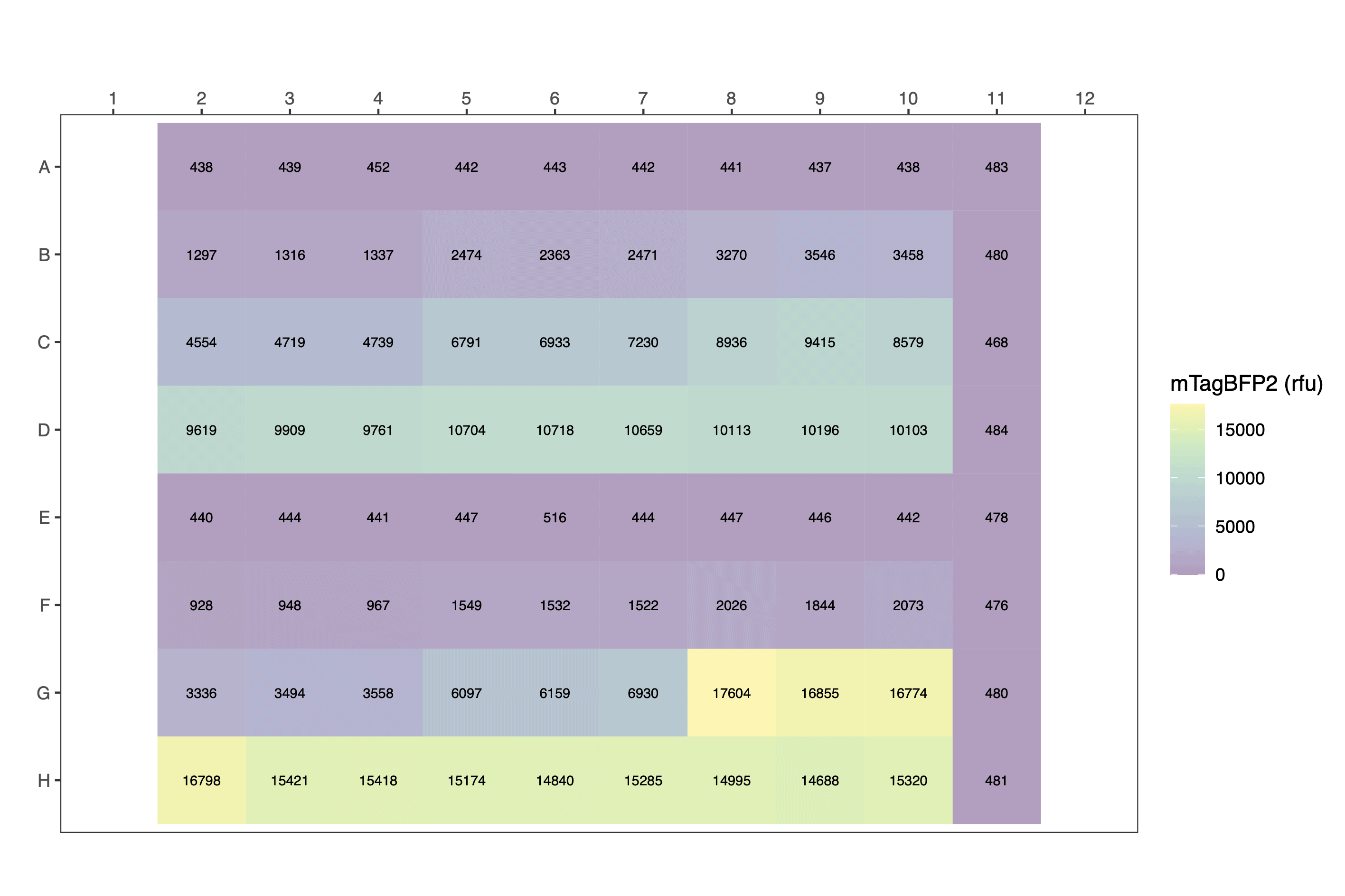
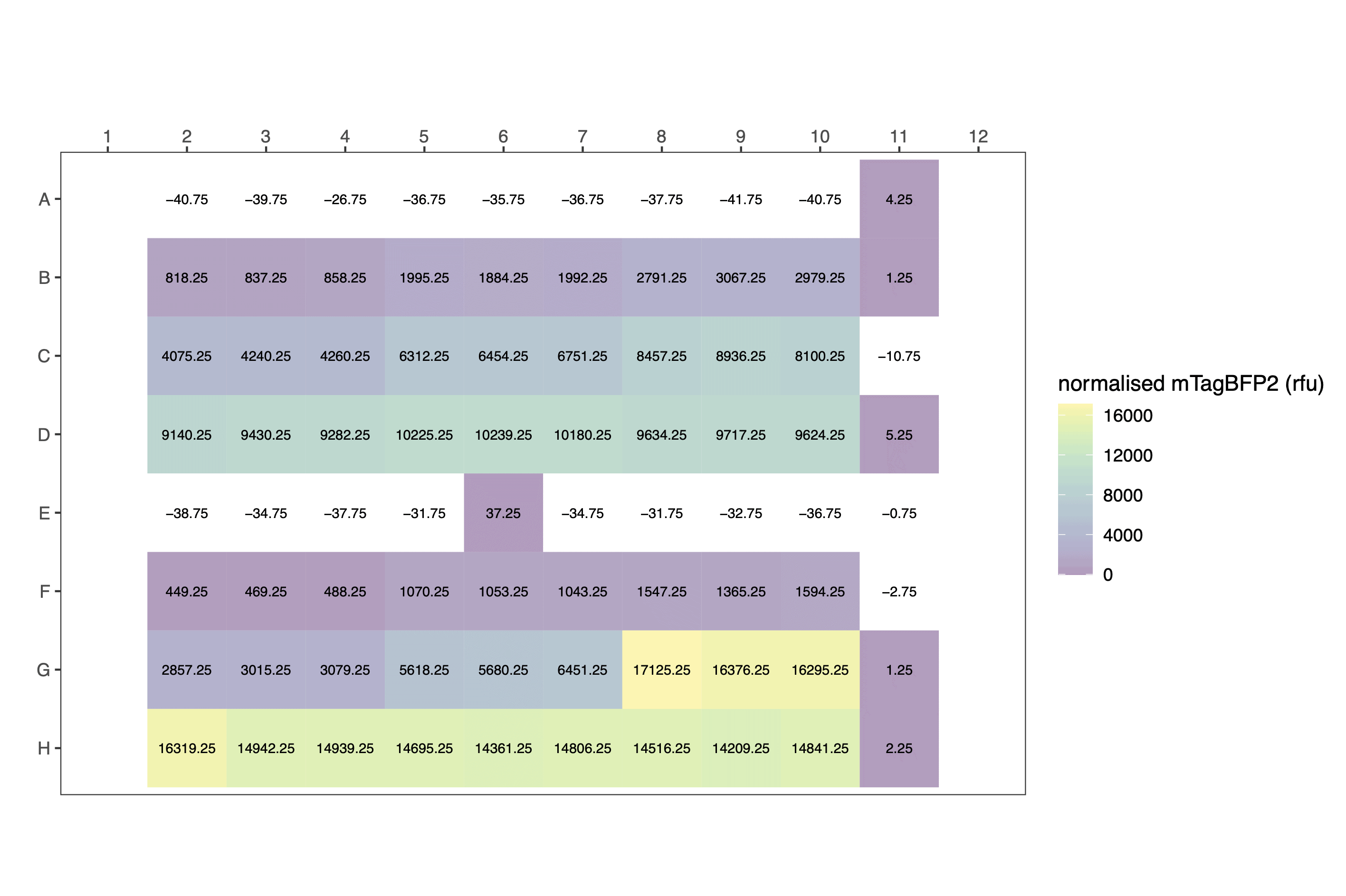
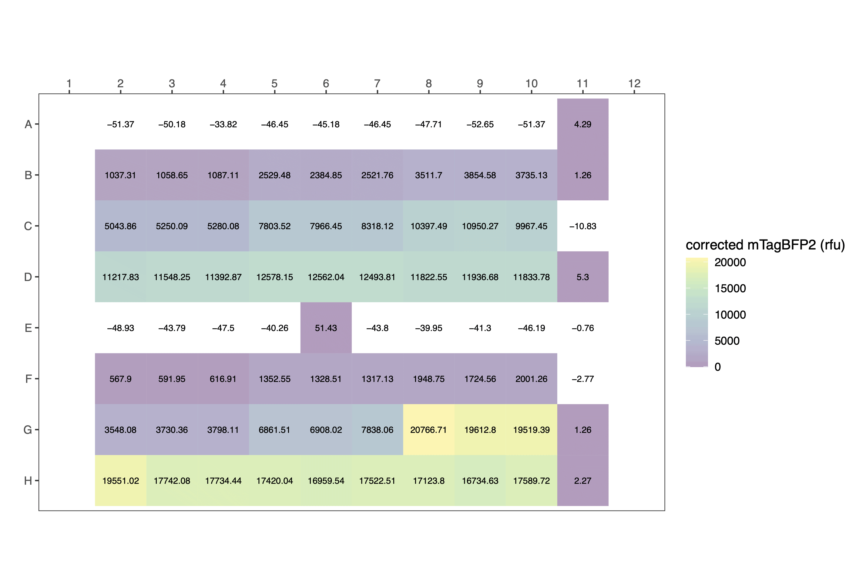
The plot formats are heatmap styled.
Raw:
Calculate per cell values
calc_fppercell() can be used to estimate molecules per
cell.
pc_data_mTagBFP2 <- calc_fppercell(
data_csv = "experiment_analysis/example_experiment2_parsed_processed.csv",
timecourse = FALSE,
flu_channels = c("blueblue"),
flu_labels = c("mTagBFP2"),
remove_wells = c("A11", "B11", "C11", "D11", "E11", "F11", "G11", "H11", # media
"A1", "B1", "C1", "D1", "E1", "F1", "G1", "H1",
"A12", "B12", "C12", "D12", "E12", "F12", "G12", "H12"), # empty wells
get_rfu_od = FALSE,
get_mol_cell = TRUE,
outfolder = "experiment_analysis"
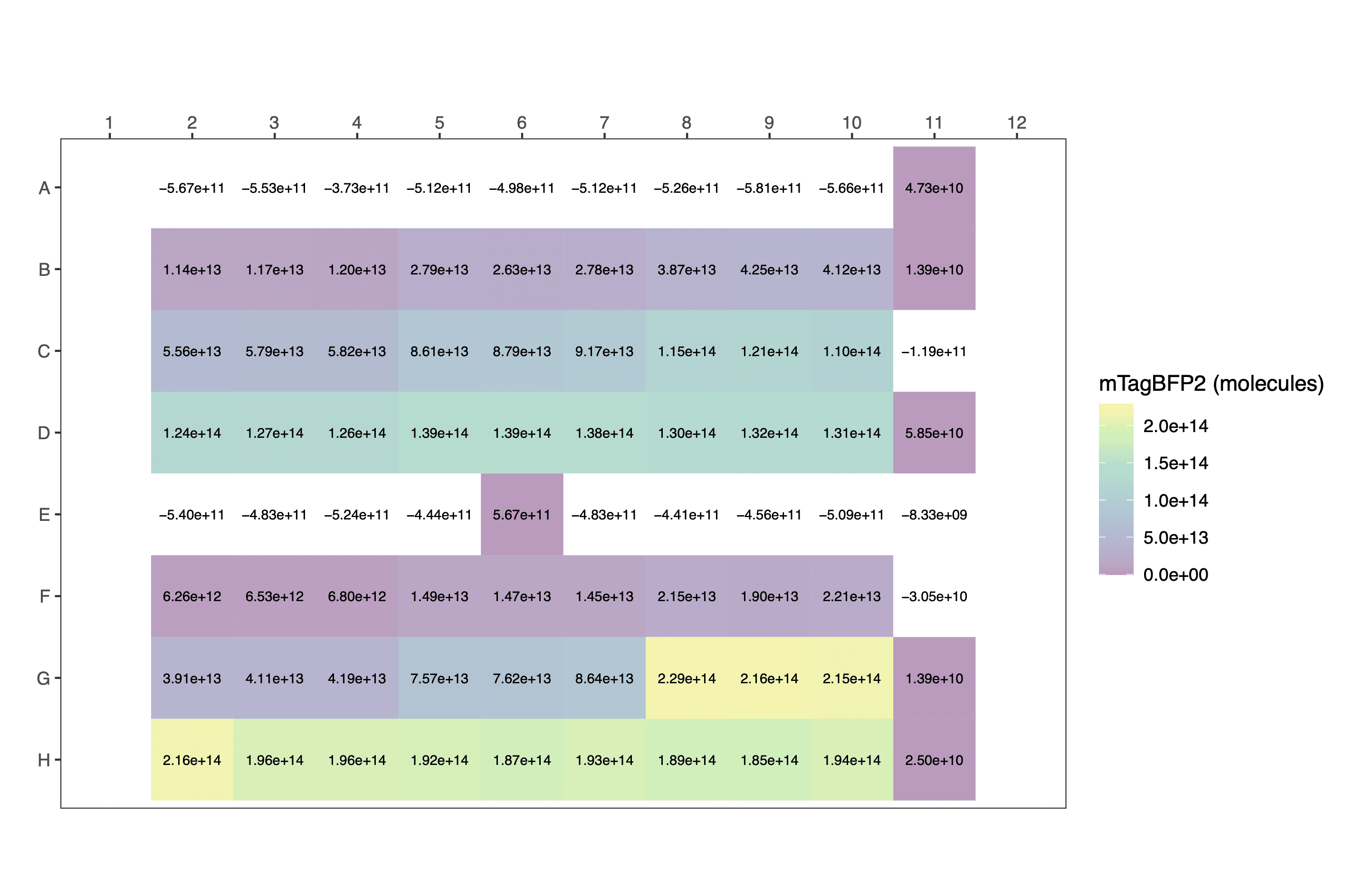
)The following differences apply for calc_fppercell() and
calc_fpconc() where timecourse = FALSE:
- No requirement for a column labelled
time. - Plots are in heatmap format, rather than line plot format.
View a fragment of the dataframe to check it:
data_to_display <- pc_data_mTagBFP2 |>
  dplyr::select(plasmid, ara_pc, OD700, calibrated_OD, blueblue, calibrated_mTagBFP2, calibratedmTagBFP2_perCell)
data_to_display[c(13:15,19:21,25:27,31:33),]| plasmid | ara_pc | OD700 | calibrated_OD | blueblue | calibrated_mTagBFP2 | calibratedmTagBFP2_perCell |
|---|---|---|---|---|---|---|
| pS361_ara_mTagBFP2 | 1e-04 | 0.6108 | 527156900 | 2474 | 2.789567e+13 | 52917.21 |
| pS361_ara_mTagBFP2 | 1e-04 | 0.6051 | 521427753 | 2363 | 2.630071e+13 | 50439.79 |
| pS361_ara_mTagBFP2 | 1e-04 | 0.6054 | 521729287 | 2471 | 2.781060e+13 | 53304.65 |
| pS361_ara_mTagBFP2 | 1e-03 | 0.5315 | 447451400 | 4554 | 5.562491e+13 | 124314.97 |
| pS361_ara_mTagBFP2 | 1e-03 | 0.5327 | 448657536 | 4719 | 5.789930e+13 | 129050.10 |
| pS361_ara_mTagBFP2 | 1e-03 | 0.5358 | 451773388 | 4739 | 5.822995e+13 | 128891.95 |
| pS361_ara_mTagBFP2 | 1e-02 | 0.5109 | 426746062 | 8936 | 1.146661e+14 | 268698.57 |
| pS361_ara_mTagBFP2 | 1e-02 | 0.5010 | 416795439 | 9415 | 1.207623e+14 | 289739.89 |
| pS361_ara_mTagBFP2 | 1e-02 | 0.5136 | 429459869 | 8579 | 1.099235e+14 | 255957.51 |
| pS361_ara_mTagBFP2 | 1e-01 | 0.5126 | 428454755 | 10704 | 1.387149e+14 | 323756.21 |
| pS361_ara_mTagBFP2 | 1e-01 | 0.5046 | 420413847 | 10718 | 1.385372e+14 | 329525.79 |
| pS361_ara_mTagBFP2 | 1e-01 | 0.5056 | 421418961 | 10659 | 1.377848e+14 | 326954.44 |
Again, output plots are heatmaps.
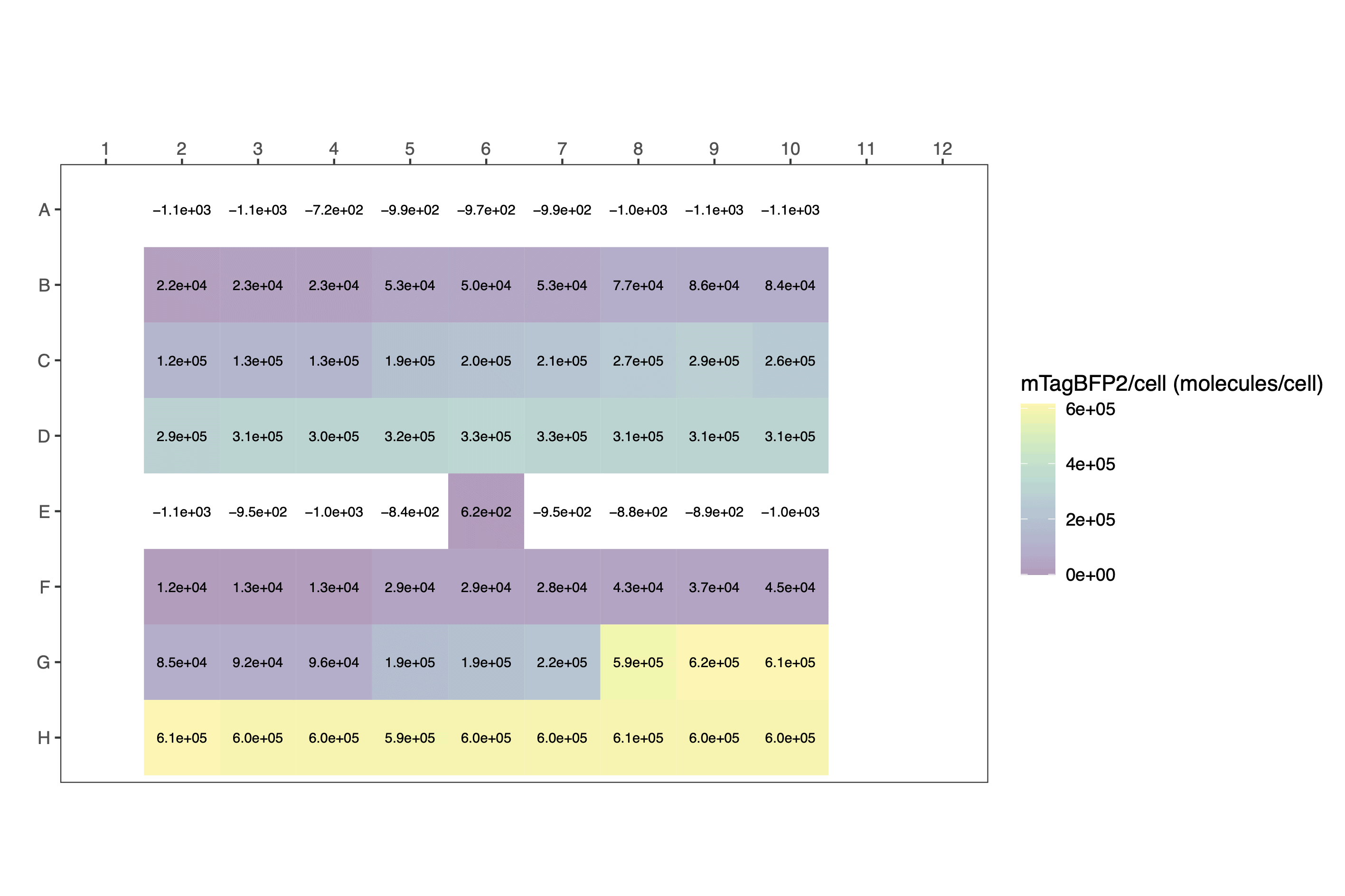
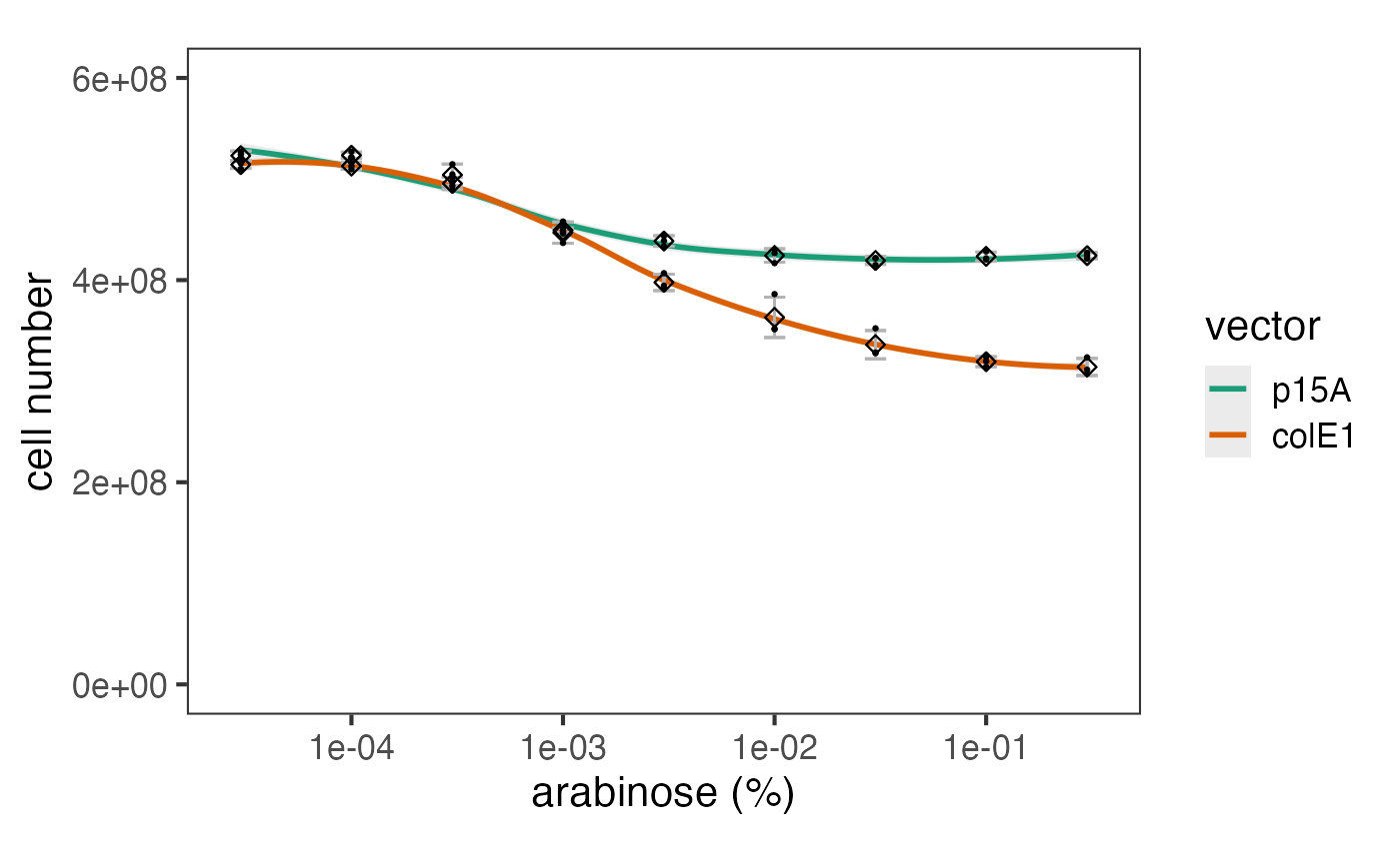
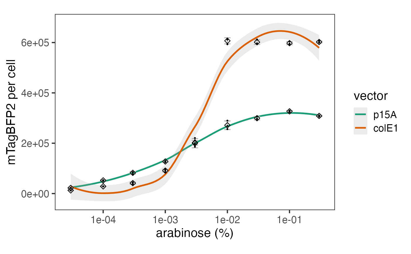
The data can be plotted downstream as a bar chart or similar.