Experiments III: Cell-Free Fluorescence

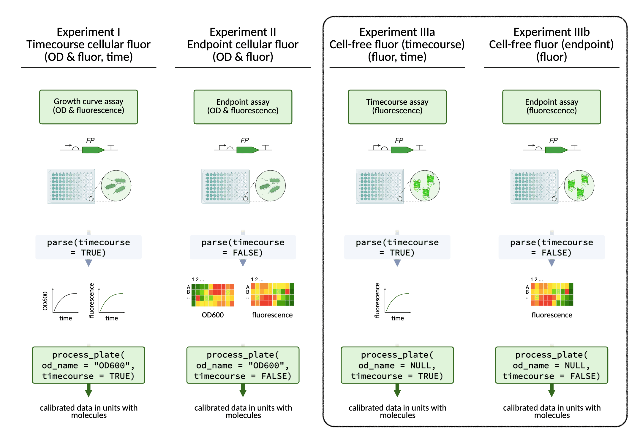
In addition to cellular fluorescence data, cell-free fluorescence data can also be processed with FPCountR, using the same functions. Just apply the argument od_name = NULL.

Processing data from cell-free fluorescent protein experiments

library(fpcountr)

Example for cell-free data

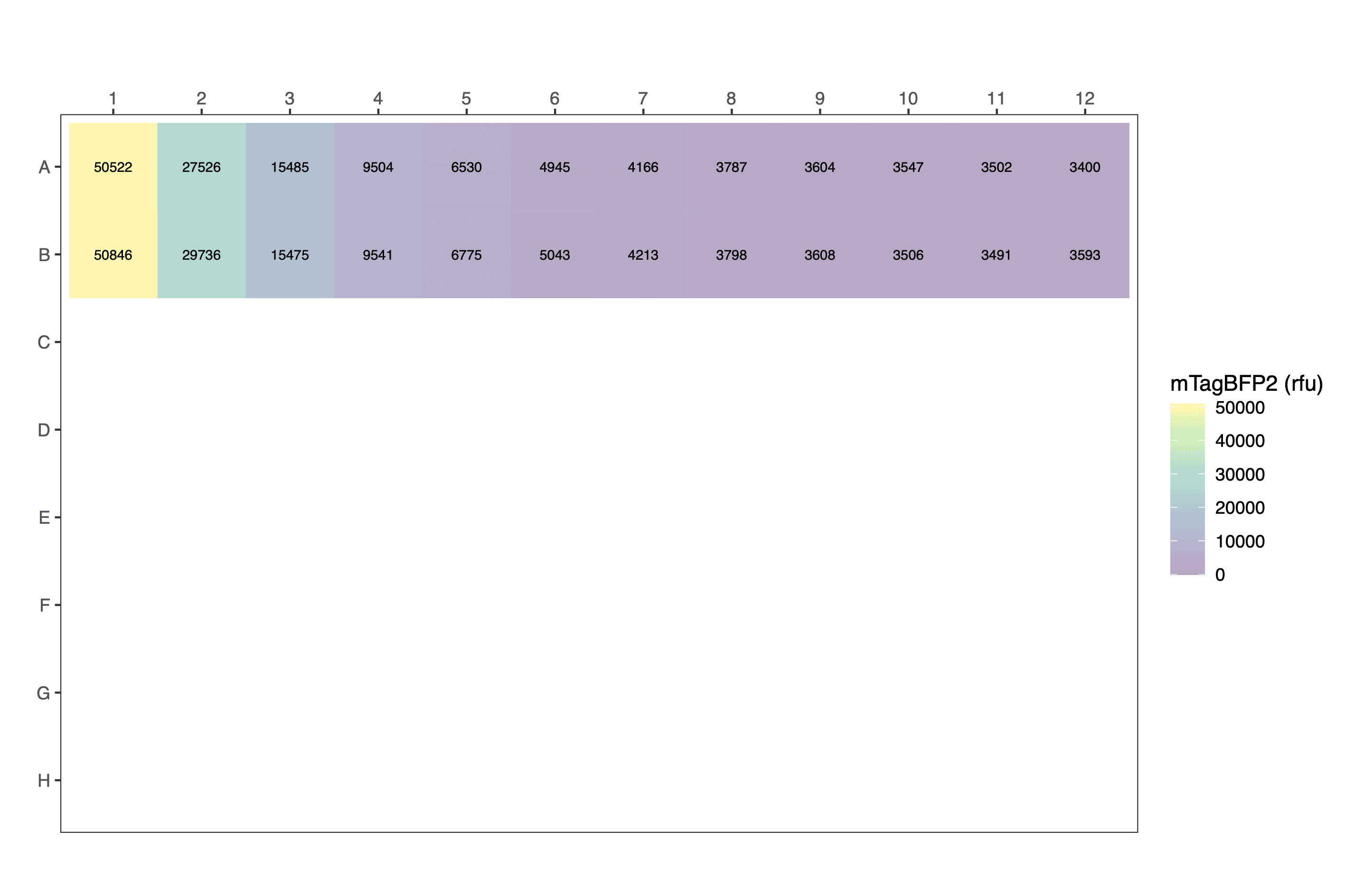
Let’s consider an example in which cell-free fluorescence was measured in vitro. For this we will use a dilution series of mTagBFP2, which was done with purified protein. This data has already been parsed. With conversion factors for calibrating mTagBFP2 fluorescence in hand, we are ready to process the experimental data.

parsed_data <- read.csv("data/example_fluorescence_simple_parsed.csv")
parsed_data[1:24,] # view a fragment of the dataframe

protein	replicate	volume	dilution	well	blueblue090	row	column
mTagBFP2	1	200	1.000000000	A1	50522	A	1
mTagBFP2	1	200	0.500000000	A2	27526	A	2
mTagBFP2	1	200	0.250000000	A3	15485	A	3
mTagBFP2	1	200	0.125000000	A4	9504	A	4
mTagBFP2	1	200	0.062500000	A5	6530	A	5
mTagBFP2	1	200	0.031250000	A6	4945	A	6
mTagBFP2	1	200	0.015625000	A7	4166	A	7
mTagBFP2	1	200	0.007812500	A8	3787	A	8
mTagBFP2	1	200	0.003906250	A9	3604	A	9
mTagBFP2	1	200	0.001953125	A10	3547	A	10
mTagBFP2	1	200	0.000976563	A11	3502	A	11
none	1	200	0.000000000	A12	3400	A	12
mTagBFP2	2	200	1.000000000	B1	50846	B	1
mTagBFP2	2	200	0.500000000	B2	29736	B	2
mTagBFP2	2	200	0.250000000	B3	15475	B	3
mTagBFP2	2	200	0.125000000	B4	9541	B	4
mTagBFP2	2	200	0.062500000	B5	6775	B	5
mTagBFP2	2	200	0.031250000	B6	5043	B	6
mTagBFP2	2	200	0.015625000	B7	4213	B	7
mTagBFP2	2	200	0.007812500	B8	3798	B	8
mTagBFP2	2	200	0.003906250	B9	3608	B	9
mTagBFP2	2	200	0.001953125	B10	3506	B	10
mTagBFP2	2	200	0.000976563	B11	3491	B	11
none	2	200	0.000000000	B12	3593	B	12

Process data

Process the experimental data using process_plate().

processed_data <- process_plate(
  data_csv = "data/example_fluorescence_simple_parsed.csv",
  blank_well = c("A12", "B12"),
  
  # timecourse
  timecourse = FALSE, ### Note requirement to declare `timecourse = FALSE`
  
  # od
  od_name = NULL, ### Note requirement to declare `od_name = NULL`
  
  # fluorescence labels
  flu_channels = c("blueblue090"),
  flu_channels_rename = c("blueblue"),
  
  # correction
  do_quench_correction = FALSE, ### Note that quench correction corrects for cells masking fluorescent signal and is not required
  
  # calibrations
  do_calibrate = TRUE,
  instr = "spark1",
  flu_slugs = c("mTagBFP2"),
  flu_gains = c(90),
  flu_labels = c("mTagBFP2"),
  
  # conversion factors
  od_coeffs_csv = "conversion_factors/od_conversion_factors_assembled.csv",
  fluor_coeffs_csv = "conversion_factors/fp_conversion_factors_assembled.csv",
  
  # background autofluorescence subtraction
  af_model = NULL, ### Note this is a requirement for `timecourse = FALSE`
  
  outfolder = "experiment_analysis"
)

The arguments are described in the ‘Get Started’ vignette. The output CSV is similar.

The following differences apply for process_plate() where od_name = NULL:

• No requirement for a column labelled OD600, OD700 or similar.
• Plots for OD and cell number are not produced.
• Autofluorescence correction does not apply, as autofluorescence is a properly of cells.
• Quench correction does not apply, as this corrects for cellular interference with fluorescence signals.

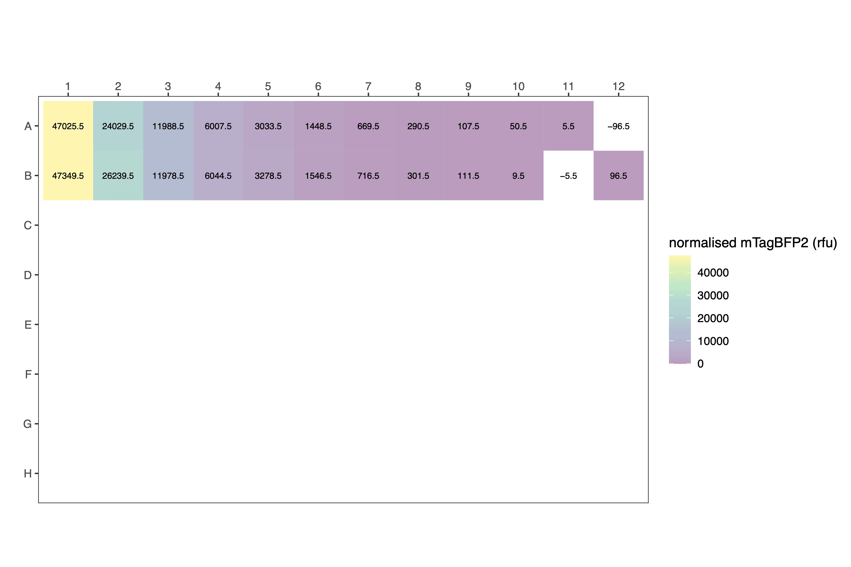
processed_data[1:12,c(1,4,5,6,9,10)] # view a fragment of the dataframe

protein	dilution	well	blueblue	normalised_blueblue	calibrated_mTagBFP2
mTagBFP2	1.000000000	A1	50522	47025.5	2.972140e+13
mTagBFP2	0.500000000	A2	27526	24029.5	1.518730e+13
mTagBFP2	0.250000000	A3	15485	11988.5	7.577059e+12
mTagBFP2	0.125000000	A4	9504	6007.5	3.796904e+12
mTagBFP2	0.062500000	A5	6530	3033.5	1.917255e+12
mTagBFP2	0.031250000	A6	4945	1448.5	9.154916e+11
mTagBFP2	0.015625000	A7	4166	669.5	4.231423e+11
mTagBFP2	0.007812500	A8	3787	290.5	1.836039e+11
mTagBFP2	0.003906250	A9	3604	107.5	6.794294e+10
mTagBFP2	0.001953125	A10	3547	50.5	3.191738e+10
mTagBFP2	0.000976563	A11	3502	5.5	3.476150e+09
none	0.000000000	A12	3400	-96.5	-6.099064e+10

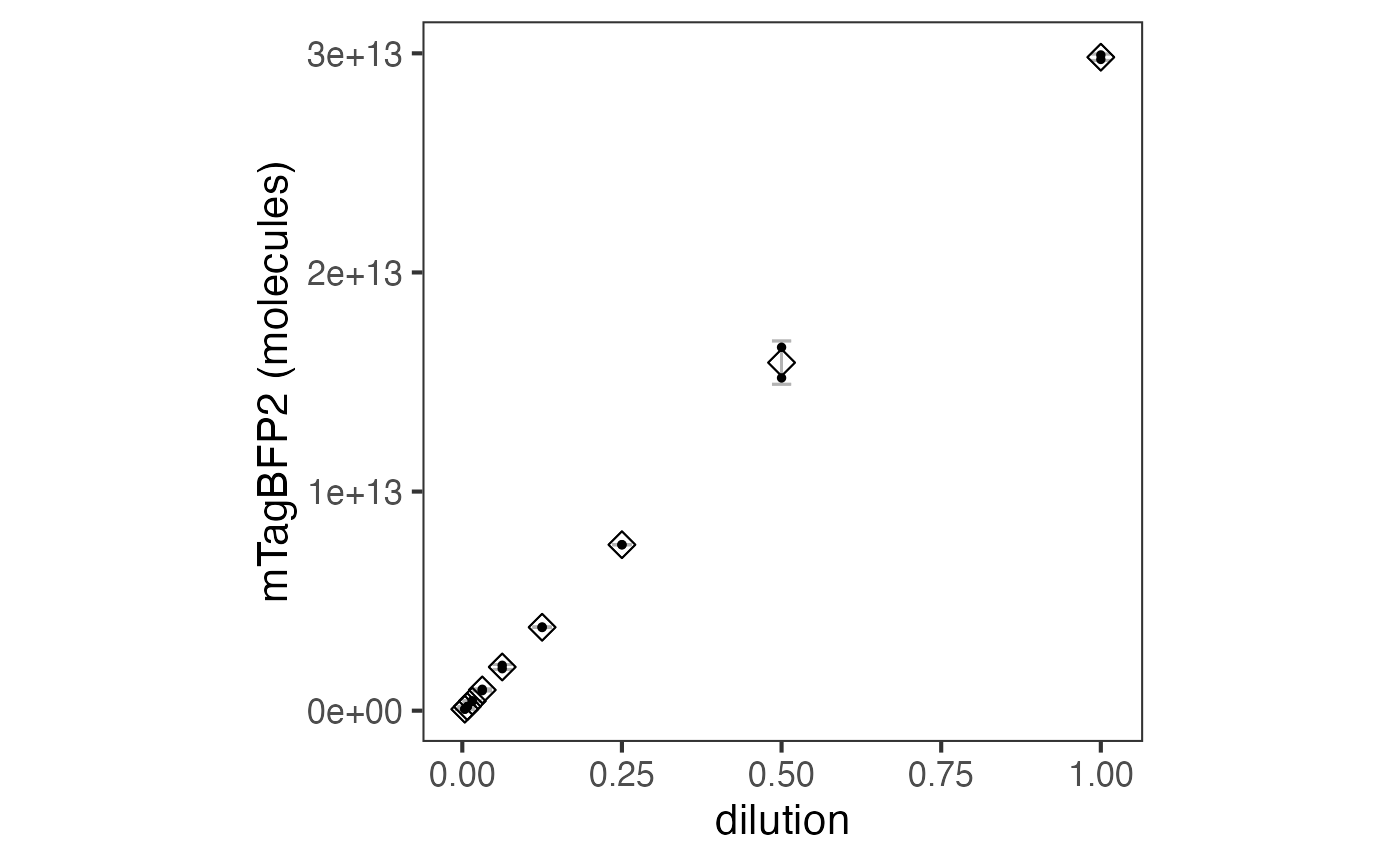
Output plot formats depend on whether the data is endpoint or timecourse/kinetic data.

Raw:

Normalised:

Calibrated:

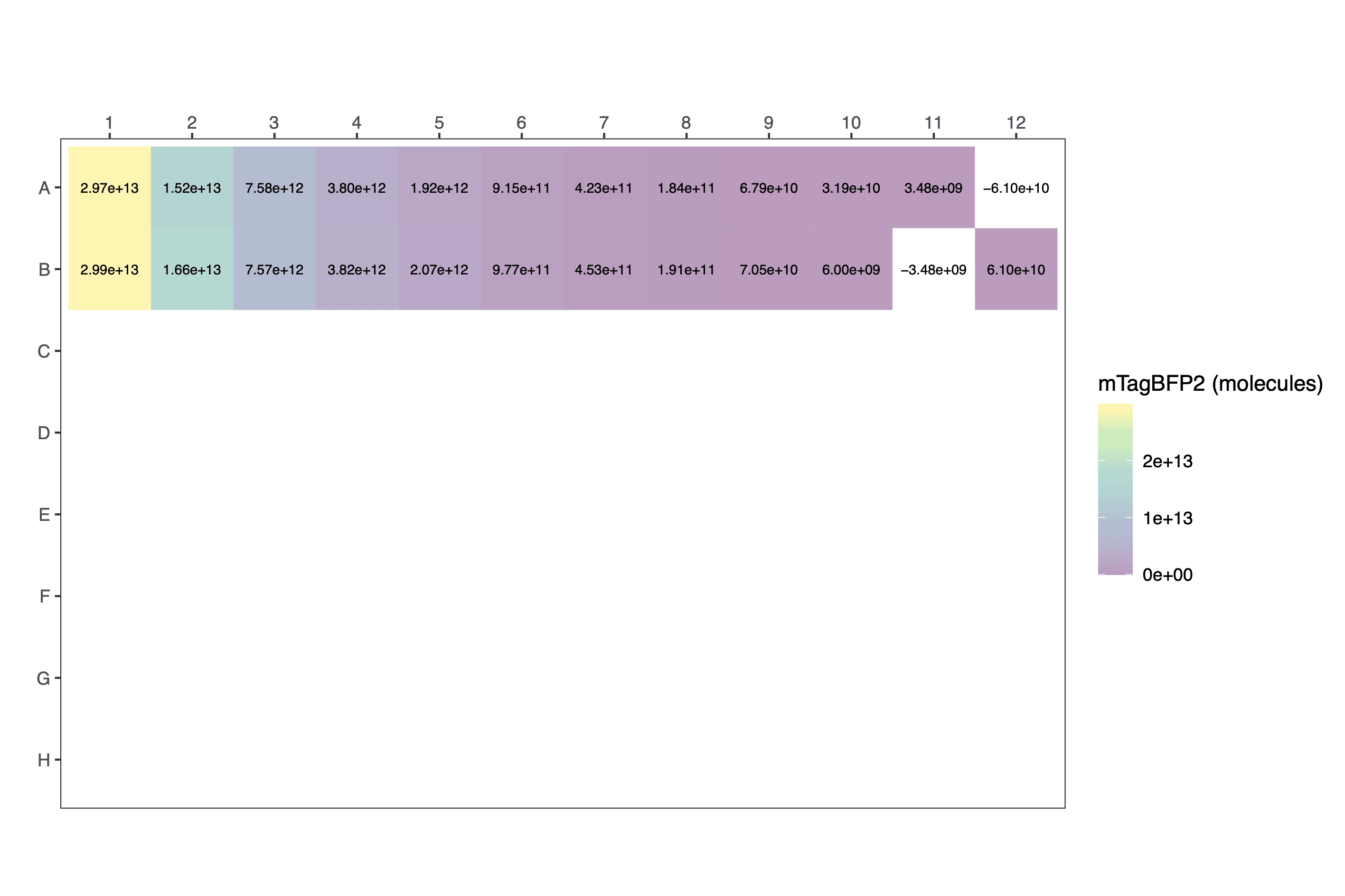
The data can be plotted downstream as a scatter plot or similar.